Window functions in PySpark
Running totals, ranks, lag/lead — the same window functions you know from SQL, in the DataFrame API. The pattern that solves half of analytics work.
Written and reviewed by Shreyash Prashu Last reviewed
What you'll learn
- The Window.partitionBy().orderBy() pattern
- The five functions you'll use weekly: row_number, rank, lag, lead, sum-with-frame
- Frames — rowsBetween for cumulative ops; rangeBetween for time windows
Before you start
The last lesson left us with two tools that can’t reach a certain kind of question. A join combines rows across
tables; a groupBy collapses rows within one — but neither can answer “what was this user’s running total up to
this order?”
Nor can either answer “where does each row rank in its country?” Those need, for one row, context from its neighbours, with the original rows surviving. We asked for the operation that lives in exactly that gap. This is it.
If you’ve read the SQL window functions lesson, the PySpark version is the same idea with slightly more verbose syntax. A window function computes an aggregate (sum, rank, lag, etc.) without collapsing rows — each input row gets one output row.
In analytics, this is the pattern that solves:
- running totals
- deduplication
- top-N-per-group
- time-since-last-event
You’ll use it every week.
The pattern
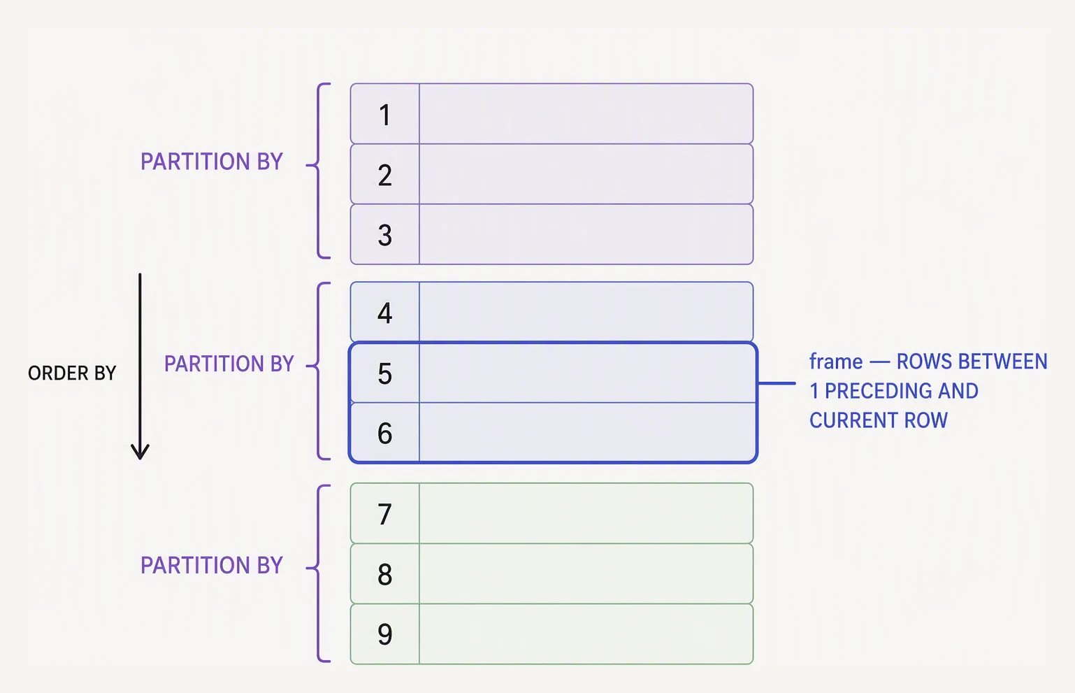
Partition picks the group, order sorts it, the frame picks which rows count.
Every window function in PySpark uses the same three pieces:
from pyspark.sql import Window
from pyspark.sql import functions as F

w = Window.partitionBy("user_id").orderBy("order_date")

df.withColumn("running_total", F.sum("amount").over(w))
Three pieces:
partitionBy— split rows into independent groups (likeGROUP BY, but rows stay)orderBy— order rows within each partition.over(w)— apply the function over the window spec
Two pieces are optional:
- Skip
partitionByto compute over the whole DataFrame as one window - Skip
orderByfor unordered aggregates (e.g., partition-wide sum)
Running total per user
The textbook case:
from pyspark.sql import SparkSession, Window
from pyspark.sql import functions as F

spark = SparkSession.builder.getOrCreate()
orders = spark.read.parquet("s3://bucket/orders/")

w = Window.partitionBy("user_id").orderBy("order_date")

per_user = orders.withColumn(
    "running_total",
    F.sum("amount").over(w),
)

per_user.show()
For every order, you get the cumulative amount for that user up
through that order date. No GROUP BY, no row collapse.
Ranking — row_number, rank, dense_rank
The three ranking functions, just like SQL:
w = Window.partitionBy("country").orderBy(F.desc("spend"))

ranked = (users
    .withColumn("rn",  F.row_number().over(w))
    .withColumn("rk",  F.rank().over(w))
    .withColumn("drk", F.dense_rank().over(w)))
Same tie-breaking rules:
| Function | Ties behavior |
|---|---|
row_number() | Unique sequential (1, 2, 3, 4) — ties broken arbitrarily |
rank() | Tied rows share rank; next rank skips (1, 2, 2, 4) |
dense_rank() | Tied rows share rank; next rank doesn’t skip (1, 2, 2, 3) |
The most-used pattern in real work is top-N per group:
# Top 3 spenders per country
w = Window.partitionBy("country").orderBy(F.desc("spend"))

top3 = (users.withColumn("rn", F.row_number().over(w))
             .filter(F.col("rn") <= 3)
             .drop("rn"))
Same wrap-and-filter trick as SQL: compute the rank in a column, then filter on it.
lag and lead — the “previous row” trick
lag(col, n) gives you the value of col from n rows back within
the window. lead(col, n) gives you n rows forward.
w = Window.partitionBy("user_id").orderBy("order_date")

orders_with_prev = orders.withColumn(
    "prev_order_date",
    F.lag("order_date", 1).over(w),
).withColumn(
    "days_since_last",
    F.datediff(F.col("order_date"), F.col("prev_order_date")),
)
For every order, you get the previous order date for the same user and the gap in days. This is the foundation of:
- churn analysis
- session detection
- user-journey work
lag also takes a third argument: the default when there’s no
previous row.
F.lag("amount", 1, 0).over(w) # use 0 if no previous rowFrames — rowsBetween and rangeBetween
By default a partitionBy().orderBy() window includes all rows from
the start of the partition up to and including the current row.
That’s the “running total” frame.
You control the frame explicitly with rowsBetween or rangeBetween:
# Last 7 orders (the 6 before + the current one)
w_7 = Window.partitionBy("user_id").orderBy("order_date") \
            .rowsBetween(-6, Window.currentRow)

# Full per-user partition (no order needed)
w_all = Window.partitionBy("user_id") \
              .rowsBetween(Window.unboundedPreceding, Window.unboundedFollowing)

orders.withColumn("last_7_total", F.sum("amount").over(w_7))
The named constants:
| Constant | Meaning |
|---|---|
Window.unboundedPreceding | Start of partition |
Window.unboundedFollowing | End of partition |
Window.currentRow | The current row |
| Negative integer | N rows before current |
| Positive integer | N rows after current |
rowsBetween counts by position. rangeBetween counts by the
value of the orderBy column — useful for time windows where
rows may be uneven:
# All orders in the last 30 days (by date value, not row count)
w_30d = (Window.partitionBy("user_id")
               .orderBy(F.col("order_date").cast("timestamp").cast("long"))
.rangeBetween(-30 * 86400, 0)) # seconds in 30 daysA real example — sessionizing events
Sessionization is “split a user’s events into sessions, where a new session starts after 30 minutes of inactivity.” It’s pure window-function territory:
session_window = Window.partitionBy("user_id").orderBy("event_at")

sessioned = (events
    .withColumn("prev_event", F.lag("event_at").over(session_window))
    .withColumn("gap_sec",
        F.unix_timestamp("event_at") - F.unix_timestamp("prev_event"))
    .withColumn("new_session", (F.col("gap_sec") > 30 * 60).cast("int"))
    # coalesce handles the first event per user: lag returns NULL → gap_sec
    # is NULL → new_session is NULL; treat it as 0 (start of first session).
    .withColumn("session_id",
        F.sum(F.coalesce(F.col("new_session"), F.lit(0))).over(session_window)))
That’s:
- For each event, find the previous event’s timestamp
- Compute the gap in seconds
- Flag “new session” if the gap exceeds 30 minutes
- Cumulative sum of flags = the session id for that user
The same logic in raw map-reduce would be ~50 lines. In windows it’s 4 withColumn calls.
A toy windowed running total
To make the mechanics concrete:
# Toy: running total per user, ordered by date.
from collections import defaultdict

orders = [
    ("u1", "2026-01-01", 10),
    ("u2", "2026-01-01", 20),
    ("u1", "2026-01-02", 5),
    ("u1", "2026-01-03", 15),
    ("u2", "2026-01-02", 12),
    ("u2", "2026-01-04", 8),
]

# 1) Group by partition key (user_id)
partitions = defaultdict(list)
for u, d, amt in orders:
    partitions[u].append((d, amt))

# 2) Within each partition, order by date and compute running total
result = []
for u, rows in partitions.items():
    rows.sort(key=lambda r: r[0])
    total = 0
    for d, amt in rows:
        total += amt
        result.append((u, d, amt, total))

# 3) Output one row per input
for u, d, amt, total in sorted(result, key=lambda r: (r[0], r[1])):
    print(f"{u}  {d}  amt={amt:>3}  running={total}")
u1 2026-01-01 amt= 10 running=10
u1 2026-01-02 amt= 5 running=15
u1 2026-01-03 amt= 15 running=30
u2 2026-01-01 amt= 20 running=20
u2 2026-01-02 amt= 12 running=32
u2 2026-01-04 amt= 8 running=40Notice two things that are the window function. First, six rows went in and six came out — nothing collapsed, the
way a groupBy would have crushed each user to a single total.
Second, the running total restarts at each user: u1 climbs 10 → 15 → 30 while u2 independently climbs 20 → 32 →
40. That’s because partitionBy("user_id") walls the two users into separate windows, and the order-by date defines
the sweep within each.
Spark’s window engine does exactly this across thousands of users at once — partitionBy is the group, orderBy is
the sweep, and the frame (here, everything up to the current row) is what F.sum(...).over(w) accumulates.
Cost reminder
A Window.partitionBy(...) is a shuffle. Spark sends all rows
with the same partition key to one executor, just like a groupBy.
Same skew problems apply — if 80% of your rows have user_id = NULL,
that one task is going to be very slow.
If you don’t need a partition (you want a single global ordering), Spark falls back to a single-task computation, which is a different performance trap. For big global windows, consider whether you really need the global order or could partition on a coarser key.
In one breath
A window function computes an aggregate without collapsing rows — every input row gets one output row — via the
three-part Window.partitionBy(...).orderBy(...) spec plus .over(w).
partitionBy splits into independent groups (rows survive), orderBy sequences within each, and an optional
frame (rowsBetween counts positions, rangeBetween counts the order-by value, e.g. last-30-days) bounds
what’s aggregated.
The weekly toolkit is:
row_number/rank/dense_rank— the top-N-per-group “rank-then-filter” tricklag/lead— previous/next row, behind churn and sessionization- framed
sum— running totals
Remember a partitionBy is a shuffle, so a window with no
partitionBy forces the whole DataFrame onto one executor.
Practice
Before the quiz, write the top-N-per-group recipe from memory: to get the top 3 spenders per country, which window
function, which two-step “wrap and filter” pattern, and why row_number rather than rank?
Then consider the performance trap the lesson ends on: you run F.sum("x").over(Window.orderBy("date")) with no
partitionBy on a billion-row table and it crawls.
Explain exactly what Spark is forced to do, and the one change that fixes it.
Quick check
groupBy('country').sum('amount') and F.sum('amount').over(Window.partitionBy('country'))?A question to carry forward
Step back over this whole chapter and notice the one thing every operation had in common:
- select
- filter
- join
- groupBy
- rank
- lag
- running sums
You never wrote the actual computation. You named F.sum, F.row_number,
F.lag, F.datediff, and Spark supplied the logic, written in the JVM,
optimizable by Catalyst, running at full speed. The entire
pyspark.sql.functions library is a catalogue of pre-built, fast
operations.
But your real work will eventually want something that isn’t in the catalogue:
- a bespoke scoring formula
- a call to a Python ML model
- a parsing rule only you know
The instant you need your own Python logic on a column, you’ve left the world of built-in functions. The obvious move — wrap a plain Python function as a UDF — is one of the most notorious performance cliffs in Spark.
That’s because every row has to cross the boundary between the JVM and a Python process one value at a time. So the question to carry forward, the one that closes this chapter: when Spark’s built-ins run out and you must run your own Python on a billion rows, how do you do it without falling off that cliff?
That is Pandas UDFs, and it is the next lesson.
Practice this in an interview
All questionsUse SUM() OVER (ORDER BY ...) — the default frame is RANGE BETWEEN UNBOUNDED PRECEDING AND CURRENT ROW. This works correctly for strictly increasing order columns, but silently over-counts when multiple rows share the same ORDER BY value because the RANGE default includes all peers.
rolling() computes statistics over a fixed-size sliding window, discarding data outside the window; expanding() grows the window from the first row to the current row, equivalent to an ever-increasing cumulative calculation. Both return objects you chain .mean(), .sum(), .std(), or a custom .apply() onto.
Window functions are evaluated in the SELECT phase, after WHERE and HAVING have already filtered rows. Referencing a window function alias in WHERE causes a syntax or evaluation-order error. The fix is to wrap the query in a CTE or subquery so the outer query can filter on the computed window value.
pandas operates in-memory on a single machine, making it fast and simple for datasets under a few gigabytes. Spark distributes computation across a cluster, handles terabyte-scale data, and integrates with cloud storage — but adds significant overhead for small data. The crossover point is roughly when your data no longer fits in RAM or when processing time on a single machine becomes unacceptable.