Reading explain plans
.explain() shows the physical plan Spark will run. Learn to read it top-down and you can debug almost any slow job — find the shuffle, find the broadcast, find the scan.
Written and reviewed by Shreyash Prashu Last reviewed
What you'll learn
- The five
.explain()modes — when to use each - How to read a physical plan top-down
- The two questions every senior engineer asks at a plan: where's the shuffle? is the right table broadcast?
Before you start
The last lesson asked you to take Catalyst on faith. “It pushed the filter down,” “it pruned to 5 columns,” “it chose a broadcast” — every claim was asserted through a hand-written before/after sketch.
We ended by insisting that in production you cannot take it on faith: you force a broadcast and must confirm it broadcast, you expect a pushdown and must confirm the scan skipped row groups. The proof lives in one output we kept glancing at and never deciphering. This lesson teaches you to read it.
df.explain() is the most valuable line of code in your PySpark
debugging toolkit. It shows you what Spark will actually run —
which is often quite different from what you wrote. Crucially, calling
.explain() does not execute the query; it only prints the plan.
Learn to read it and you’ve earned half a senior engineer’s badge.
The five modes
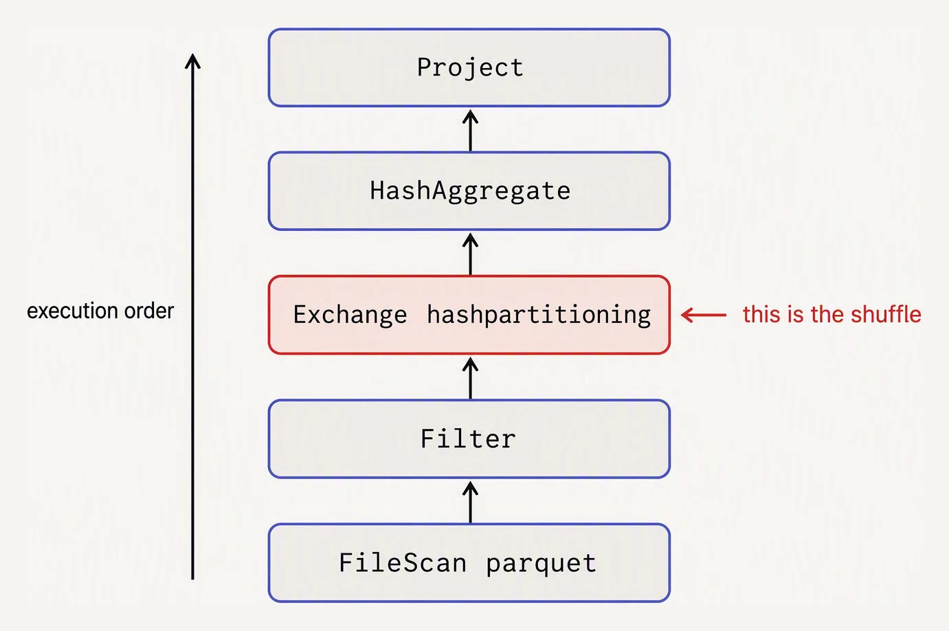
Read it bottom-up: the leaves run first.
.explain() accepts a mode argument. The five modes give you
different levels of detail.
| Mode | Shows | When to use |
|---|---|---|
"simple" (default) | Just the physical plan | Quick sanity check |
"extended" | All four plans (parsed, analyzed, optimized, physical) | See what Catalyst rewrote |
"formatted" | Physical plan with detail blocks below | Day-to-day debugging — best for humans |
"codegen" | The generated Java code | Only if you’re tracing a perf mystery |
"cost" | Plan with cost estimates | Joins where Spark’s strategy choice looks wrong |
The one you’ll use 95% of the time is formatted:
df.explain(mode="formatted")Reading a physical plan top-down
A physical plan reads top-down = downstream-to-upstream. The operator at the top runs last; the scan at the bottom runs first.
== Physical Plan ==
AdaptiveSparkPlan isFinalPlan=false
+- Project [user_id, country, revenue]
   +- HashAggregate(keys=[user_id, country], functions=[sum(amount)])
      +- Exchange hashpartitioning(user_id, country, 200)
         +- HashAggregate(keys=[user_id, country], functions=[partial_sum(amount)])
            +- BroadcastHashJoin [user_id], [user_id], Inner
               :- Filter (status = 'PAID')
               :  +- FileScan parquet [user_id, country, amount, status]
               +- BroadcastExchange HashedRelationBroadcastMode
                  +- FileScan parquet users [user_id]
Read it bottom-to-top:
- FileScan parquet [user_id, country, amount, status] — read the orders file. Notice only 4 columns are read (column pruning).
- Filter (status = ‘PAID’) — apply the status filter (probably already pushed down into the scan as well).
- BroadcastExchange + FileScan parquet users — read the users table and broadcast it to every executor.
- BroadcastHashJoin — join orders with the broadcasted users by user_id. No shuffle of the big side.
- HashAggregate (partial) — partial aggregation per partition.
- Exchange hashpartitioning(…) — the shuffle. Repartition by (user_id, country) so all rows with the same key meet.
- HashAggregate (final) — final aggregation after the shuffle.
- Project — select the output columns.
That’s a complete read. Once you can do this, you can debug.
Read an execution plan: operators, shuffles, and row estimates
The query orders.filter(status=PAID).groupBy(country).agg(sum(amount)) below is shown as a physical plan. Execution flows bottom-up — the scan at the bottom runs first. Click any node to see estimated vs actual rows. Toggle filter pushdown to see how moving the scan earlier shrinks the shuffle.
The optimizer keeps the filter above the scan. The scan reads all 10 million rows before filtering.
Execution order: bottom (scan, step 1) to top (project, last step)
The two questions every senior engineer asks
When opening any explain plan, two questions matter:
Q1: Where’s the shuffle?
Find every line starting with Exchange. Each Exchange is a
shuffle — your most expensive operation. Common Exchange types:
Exchange hashpartitioning(...)— full shuffle for a join or aggregationExchange RoundRobinPartitioning— fromrepartition(N)without a keyExchange SinglePartition— collecting to one executor (often a global orderBy — usually slow)
If there are more Exchanges than you expect, you’ve got a chance to optimize.
Q2: Is the right table broadcast?
Find every BroadcastExchange. The table below it is the one being
broadcast. Check that it’s the small side of the join.
BroadcastHashJoinwith the small table broadcast: goodSortMergeJoinwith a small dim table: suspicious — should probably be broadcastBroadcastHashJoinwith a large table broadcast: bad — risk of executor OOM
If a small table isn’t broadcasting when it should, add an explicit hint:
fact.join(F.broadcast(small_dim), "key")A walkthrough of mode="formatted"
formatted is the most readable mode. It splits the plan into a
numbered tree at the top and per-operator detail blocks below.
(orders
  .filter(F.col("status") == "PAID")
  .join(F.broadcast(users), "user_id")
  .groupBy("country")
  .agg(F.sum("amount").alias("revenue"))
  .explain(mode="formatted"))
Output (abbreviated):
== Physical Plan ==
* HashAggregate (8)
+- Exchange (7)
   +- * HashAggregate (6)
      +- * Project (5)
         +- * BroadcastHashJoin Inner (4)
            :- * Filter (2)
            :  +- * ColumnarToRow (1)
            :     +- BatchScan parquet orders (0)
            +- BroadcastExchange (3)
               +- * ColumnarToRow
                  +- BatchScan parquet users

(0) BatchScan parquet orders
PushedFilters: [IsNotNull(status), EqualTo(status, PAID)]
ReadSchema: struct<user_id:bigint, status:string, amount:double>

(2) Filter
Predicate: (status = 'PAID')

(4) BroadcastHashJoin
Join condition: (user_id = user_id)
BuildSide: BuildRight    -- broadcasting the RIGHT (users) — good

(7) Exchange
Partitioning: hashpartitioning(country, 200)
The detail blocks at the bottom tell you:
- What columns are read (ReadSchema) — confirms pruning works
- What filters were pushed down (PushedFilters) — confirms predicate pushdown
- Which side of the join is broadcast (BuildSide) — broadcast confirmed
- What partitioning the shuffle uses — for tuning shuffle count
Spotting expensive patterns
| Plan pattern | Means | Fix |
|---|---|---|
Multiple Exchange lines | Multiple shuffles | Combine groupBys, partition once and re-use |
SortMergeJoin with small side | Broadcast was missed | Add F.broadcast(small_df) hint |
Exchange SinglePartition | Forcing data to one executor (global sort) | Avoid global orderBy unless you must |
Many small FileScans | Too many small files | Compact (Delta OPTIMIZE, or repartition before write) |
BatchEvalPython | Python UDF | Replace with built-in or pandas UDF |
No PushedFilters for a known filter | Filter not pushed down | Often: source is CSV/JSON (not Parquet) |
The number of Exchange lines in your plan is a rough proxy for cost.
A two-stage job has one Exchange. A complex aggregation might have
three. If you see seven, look closer.
A real debug session
You have a query that’s slow. You suspect a missing broadcast. The flow:
# Look at the plan
slow_df.explain(mode="formatted")

# Spot: SortMergeJoin between orders (500GB) and products (40MB)
# Conclusion: products should be broadcast but isn't

# Fix: explicit broadcast hint
fixed_df = orders.join(F.broadcast(products), "product_id") \
                 .groupBy("country").sum("amount")

# Verify the new plan
fixed_df.explain(mode="formatted")
# Now shows BroadcastHashJoin — confirmed
Two .explain() calls, problem identified and fixed. Same flow for
any plan-level optimization.
A toy plan printer
The structure of a Spark plan is just a tree. You can build a toy version in pure Python:
# Print a Spark-shaped plan tree.
class Node:
    def __init__(self, name, *children, **details):
        self.name = name
        self.children = children
        self.details = details

def print_plan(node, prefix="", is_last=True):
    connector = "+- " if is_last else "+- "
    print(f"{prefix}{connector}{node.name}")
    for k, v in node.details.items():
        print(f"{prefix}{'   ' if is_last else '|  '}    {k}: {v}")
    next_prefix = prefix + ("   " if is_last else "|  ")
    for i, child in enumerate(node.children):
        print_plan(child, next_prefix, is_last=(i == len(node.children) - 1))

plan = Node("HashAggregate",
    Node("Exchange",
        Node("HashAggregate",
            Node("BroadcastHashJoin",
                Node("Filter",
                    Node("Scan orders", ReadSchema="user_id, amount, status"),
                    Predicate="status = PAID",
                ),
                Node("BroadcastExchange",
                    Node("Scan users", ReadSchema="user_id"),
                ),
                BuildSide="BuildRight",
            ),
        ),
        Partitioning="hashpartitioning(country, 200)",
    ),
)

print("== Physical Plan ==")
print_plan(plan)
== Physical Plan ==
+- HashAggregate
+- Exchange
Partitioning: hashpartitioning(country, 200)
+- HashAggregate
+- BroadcastHashJoin
BuildSide: BuildRight
+- Filter
| Predicate: status = PAID
| +- Scan orders
| ReadSchema: user_id, amount, status
+- BroadcastExchange
+- Scan users
ReadSchema: user_idRead that output as a senior engineer would, bottom-up, and every claim Catalyst made is now visible.
The two Scan leaves run first, and their ReadSchema lines prove column pruning — Scan orders reads only three columns, not all of them. The Filter carries Predicate: status = PAID, the pushdown.
The BroadcastExchange wrapping Scan users plus BuildSide: BuildRight confirms the small users table is the one being broadcast — so there’s no shuffle of orders. The single Exchange near the top, hashpartitioning(country, 200), is the one shuffle in the whole job, for the final group-by.
That’s the same tree shape Spark prints. Once you can read this one, real plans stop being intimidating walls of text and become a checklist you tick off.
In one breath
df.explain() prints what Spark will actually run without executing it, and you read the physical plan bottom-up (deepest/most-indented scans run first, the top operator last).
The day-to-day mode is "formatted" (numbered tree plus per-operator detail blocks — PushedFilters, ReadSchema, BuildSide).
A senior engineer opens any plan asking two questions: where’s the shuffle? and is the right table broadcast? Every Exchange line is one shuffle, your most expensive operation. Find BroadcastExchange/BroadcastHashJoin and check the small side is the one being shipped.
The count of Exchange lines serves as a rough cost proxy, and BatchEvalPython flags a UDF to replace.
Practice
Before the quiz, run the senior-engineer scan on the worked plan above. Point to the exact line that is the shuffle, the exact line that proves the small table broadcast (and which side), and the line that proves column pruning happened.
Then the debug reflex: you see SortMergeJoin between a 500 GB and a 40 MB table. What does that tell you? What one-line change fixes it? And how do you confirm the fix with a second .explain()?
Quick check
Exchange hashpartitioning(user_id, 200) in your plan. What does that mean?SortMergeJoin between a 500GB table and a 50MB table. What's the issue and fix?A question to carry forward
Look at the very top line of every plan in this lesson — the one we read straight past on our way down to the scans: AdaptiveSparkPlan isFinalPlan=false.
We never asked what it meant, but it’s quietly admitting something unsettling about everything we just learned to read. The plan is labelled not final. Catalyst built it before a single row was processed, from estimates — and estimates lie.
The stats are stale. The size of a table after a filter is a guess until the filter actually runs.
So the plan you just learned to verify is provisional. Spark reserves the right to look at what the data actually turns out to be — mid-job, between stages — and rewrite the rest of the plan on the spot.
A join it planned as a shuffle becomes a broadcast because one side came out tiny; a partition that ballooned gets split. That isFinalPlan=false is the optimizer admitting it will change its mind once it sees reality.
So the question to carry forward is: what is this runtime second-guesser that turns a compile-time plan into a final one?
And what does it actually do between stages to fix the estimates Catalyst got wrong? That is Adaptive Query Execution, and it is the next lesson.
Practice this in an interview
All questionsEXPLAIN shows the optimizer's chosen plan with estimated rows and costs before execution. EXPLAIN ANALYZE runs the query and overlays actual row counts and timing, letting you spot where estimates diverge from reality — bad statistics, missing indexes, or the wrong join algorithm — and target the correct fix.
A shuffle redistributes data across all executors so that rows with the same key end up on the same partition. It involves writing intermediate data to disk, transferring it over the network, and re-reading it — making it the most costly operation in a Spark job in terms of latency and I/O.
Lazy evaluation means Spark records transformations in a plan and waits for an action to execute it. That delay lets Spark optimize the complete DataFrame or RDD computation, while actions such as count, show, collect, and write trigger jobs.
The driver is a single JVM process that hosts the SparkContext, builds the DAG, schedules tasks, and coordinates results. Executors are JVM processes on worker nodes that actually run tasks and cache data. The cluster manager (YARN, Kubernetes, standalone) sits between them, allocating resources.