Joins in PySpark
Inner, left, semi, anti — and the only thing that really matters for performance: broadcast vs sort-merge. Pick the strategy and Spark stops being slow.
Written and reviewed by Shreyash Prashu Last reviewed
What you'll learn
- The six join types and when each is the right answer
- Broadcast hash join vs sort-merge join — when Spark picks each
- How to force a broadcast (and when not to)
Before you start
The last lesson made us fuss over key columns — order_id and user_id, typed LongType and nullable=False,
more carefully than the rest. We said a key only earns that fussiness when it’s about to be matched against another
table’s key, and that the matching means a shuffle. This lesson is that matching: how Spark combines two
well-typed DataFrames on a key, why the naive way is a full network shuffle, and the one trick that turns an hour
into a minute.
Joins are where Spark performance is won or lost. The same logical join can run in 30 seconds or 30 minutes depending on which physical strategy Spark picks. The good news: there are only two strategies worth knowing, and you control which one runs.
The six join types
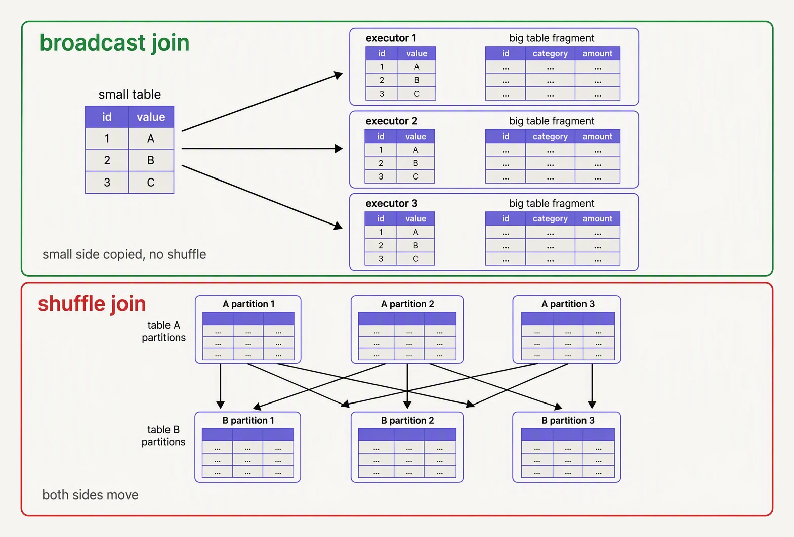
If one side fits in memory, ship it everywhere and skip the shuffle.
The semantics — what rows come out — match SQL exactly:
left.join(right, on="user_id", how="inner")     # rows that match on both sides
left.join(right, on="user_id", how="left")      # all left + matching right (or null)
left.join(right, on="user_id", how="right")     # all right + matching left (or null)
left.join(right, on="user_id", how="outer")     # union of left & right
left.join(right, on="user_id", how="left_semi") # left rows that have a match (no right cols)
left.join(right, on="user_id", how="left_anti") # left rows that have NO match
The two underrated ones:
- left_semi — like a
WHERE EXISTSfilter. “Give me users who have orders.” Faster thaninnerbecause it doesn’t expand the row count when a left row matches multiple right rows. - left_anti — like
WHERE NOT EXISTS. “Give me users who have no orders.” The most common use case is finding records that need backfilling.
# "Users with no orders" — anti join
inactive_users = users.join(orders, "user_id", "left_anti")

# "Orders from known users" — semi join
valid_orders = orders.join(users, "user_id", "left_semi")
The two physical strategies
Logically, an inner join is an inner join. Physically, Spark has two ways to compute it, and they differ by a factor of 100x in cost.
Sort-merge join (the default for big × big)
- Hash-partition both sides on the join key — shuffle
- Sort each partition by the join key
- Merge matching keys
Cost: a full shuffle of both sides. Scales fine. Slow.
Broadcast hash join (the magic for big × small)
- Send the small side to every executor (a “broadcast”)
- Build a hash table from the small side, in memory
- Scan the big side once; look each row up in the hash table
Cost: one network broadcast of the small table. No shuffle of the big side — because every executor already has the full small table in RAM, matching keys are always local. Often 10-100x faster than sort-merge for the same logical join.
The choice depends on whether the small side fits in memory.
When Spark picks each
Spark estimates the size of each side (using stats if available, or
file sizes) and picks broadcast if the smaller side is below
spark.sql.autoBroadcastJoinThreshold (default: 10MB).
spark.conf.get("spark.sql.autoBroadcastJoinThreshold")
# '10485760'  -- 10 MB
If both sides are larger than the threshold, Spark falls back to sort-merge.
This default is conservative. Many production clusters bump it to 100-500MB:
spark.conf.set("spark.sql.autoBroadcastJoinThreshold", 200 * 1024 * 1024)But careful: too high and your executors run out of memory holding the broadcast.
Forcing a broadcast with a hint
When Spark’s stats are wrong (often after filters, or with CSV sources), it picks sort-merge for a join that should have been broadcast. Force the right choice:
from pyspark.sql.functions import broadcast

# Tell Spark: broadcast the products table
joined = orders.join(broadcast(products), "product_id")
Or as a SQL hint:
SELECT /*+ BROADCAST(p) */ *
FROM orders o
JOIN products p ON o.product_id = p.product_id
This is the single most valuable performance optimization in PySpark. If you don’t read another performance lesson, learn this one.
How big is “small”?
Roughly, after compression and after you’ve selected only the columns you need:
| Table size | Strategy |
|---|---|
| Under ~10MB | Broadcast (Spark does it automatically) |
| 10MB to ~500MB | Broadcast if you can spare executor memory |
| 500MB to ~1GB | Maybe broadcast on big executors |
| Over 1GB | Sort-merge — broadcasting is risky |
The key is the size in executor memory after decompression. A 100MB Parquet file might be 1GB in memory. Check with:
small.cache().count()                # forces caching
# Now check the Storage tab in the Spark UI — shows in-memory size
Joining safely — three pitfalls
Pitfall 1: Duplicate keys explode row count
If users.user_id has duplicates, an inner join multiplies. Two
duplicates on the left × two on the right = four output rows.
# Defensive: dedupe before joining
users_unique = users.dropDuplicates(["user_id"])
orders.join(users_unique, "user_id")
Pitfall 2: Column name collisions
When both sides have a name column, the joined DF has two name
columns. Accessing joined.name is ambiguous.
# Bad
joined = orders.join(users, "user_id")
joined.select("name")          # which name? AmbiguousReferenceError

# Good — alias both sides
joined = orders.alias("o").join(users.alias("u"), "user_id")
joined.select(F.col("o.product_name"), F.col("u.name"))
Pitfall 3: NULL keys cluster (in outer joins)
For a plain inner equi-join Spark protects you: the optimizer infers
isnotnull on both join keys and prunes NULL rows before the shuffle —
they could never match anyway. The hazard is real for outer joins,
where NULL-keyed rows must be kept, and for eqNullSafe (<=>), which
treats NULL as a matchable value: there, every NULL row from both sides
hashes to the same partition. That’s instant skew.
# Outer join with many NULL keys: route the NULLs around the join
non_null = orders.filter(F.col("user_id").isNotNull()) \
                 .join(users, "user_id", "left")
null_rows = orders.filter(F.col("user_id").isNull())    # no match possible
result = non_null.unionByName(null_rows, allowMissingColumns=True)

# eqNullSafe intentionally matches NULL to NULL — and inherits the skew
orders.join(users, orders.user_id.eqNullSafe(users.user_id))
Reading the join in the plan
Always check what physical strategy Spark picked:
joined.explain(mode="formatted")Look for:
BroadcastHashJoin— the small side was broadcast (good!)SortMergeJoin— full shuffle of both sides (often optimizable)BroadcastNestedLoopJoin— Spark has no equi-join condition (e.g., a range join); it broadcasts one side and does a nested loop scan — O(n×m), very slow
If you expected a broadcast and see SortMerge, you have two options:
add a broadcast() hint, or bump the threshold.
A toy broadcast vs shuffle join
To make the cost difference concrete:
# Toy: 'broadcast' vs 'shuffle' join cost — count the network messages each needs.

big_side = [("U1", 10), ("U2", 20), ("U3", 30)] * 1000   # 3,000 rows
small_side = {"U1": "USA", "U2": "FRA", "U3": "DEU"}      # 3 rows

# --- Strategy 1: broadcast small_side ---
# 1 network message: send small_side to every executor. Big side stays in place.
broadcast_messages = 1
broadcast_join = [(u, amt, small_side.get(u)) for u, amt in big_side]
print(f"broadcast: {broadcast_messages} network msg, {len(broadcast_join):,} output rows")

# --- Strategy 2: shuffle both sides ---
# Both sides hash-partition on the join key and move over the network.
shuffle_messages = len(big_side) + len(small_side)   # rough proxy
shuffle_join = [(u, amt, small_side[u]) for u, amt in big_side if u in small_side]
print(f"shuffle:   {shuffle_messages:,} network msgs, {len(shuffle_join):,} output rows")
broadcast: 1 network msg, 3,000 output rows
shuffle: 3,003 network msgs, 3,000 output rowsBoth strategies produce the identical 3,000 rows — the result is the same join either way. The difference is entirely in the cost column: the broadcast moved one tiny payload (ship the 3-row table to everyone, then every match is a local lookup) while the shuffle moved 3,003 (every row of both sides relocated across the network to meet its key). Real Spark numbers are nuanced — compression, sort costs, partition counts — but that ratio is the whole game: when one side is small enough to broadcast, you trade a fleet-wide shuffle of a 500 GB table for a single send of a 50 MB one. Same answer, a hundredth of the work.
In one breath
PySpark’s six join types (inner, left, right, outer, left_semi, left_anti) match SQL exactly — with
the underrated left_semi (“rows that have a match”, like WHERE EXISTS, no row-multiplication) and left_anti
(“rows with no match”, for backfills) — but the thing that decides 30-seconds-vs-30-minutes is the physical
strategy: a sort-merge join shuffles both sides (the default for big × big), while a broadcast hash join
ships the small side to every executor so the big side never moves (the single biggest win, for the
fact-×-dimension shape); force it with F.broadcast(small) when Spark’s size estimate is wrong, and watch for the
three traps — duplicate keys exploding row counts, ambiguous column names, and NULL keys clustering into skew.
Practice
Before the quiz, reach for the highest-leverage move. A 500 GB fact table joins a 50 MB dimension and Spark picks
SortMergeJoin (you can see it in explain) — name the one-line fix and, using the toy’s 1-vs-3,003 message
count, explain why it removes the shuffle. Then the row-explosion trap: users.user_id has two duplicate rows
for one id and orders has three matching rows — how many output rows does an inner join produce for that id, and
what is the defensive one-liner?
Quick check
A question to carry forward
A join combines rows across two tables; a groupBy collapses rows within one. Between them they cover an
enormous amount of analytics — but notice the shape of question neither one can answer. “What was this user’s
running total up to this order?” “Where does each row rank within its country?” “How many days since this
user’s previous event?” Every one of those needs, for a single row, context from its neighbours — the rows
before it, the rows around it — and it needs the original rows to survive, not collapse into one summary per
group.
A groupBy would crush those neighbours into a single number; a join can’t reach sideways within one table. So the
question to carry forward is the operation that sits exactly in that gap: how do you compute an aggregate — a sum, a
rank, a previous value — relative to each row, across a defined window of its neighbours, without losing a single
row? That is the window function, the pattern that quietly solves half of all analytics work, and it is the
next lesson.
Practice this in an interview
All questionsA broadcast join sends a complete copy of the smaller table to every executor, so the join is done locally without any shuffle. It is the most effective single optimization for joins where one side is small enough to fit in executor memory, eliminating the most expensive network operation in a join.
pandas operates in-memory on a single machine, making it fast and simple for datasets under a few gigabytes. Spark distributes computation across a cluster, handles terabyte-scale data, and integrates with cloud storage — but adds significant overhead for small data. The crossover point is roughly when your data no longer fits in RAM or when processing time on a single machine becomes unacceptable.
repartition triggers a full shuffle to produce exactly N evenly distributed partitions and can both increase and decrease partition count. coalesce merges existing partitions on the same or nearby executors without a shuffle, but can only decrease partition count and may produce uneven partitions.
Narrow transformations compute each output partition using data from exactly one input partition — no data moves across the network. Wide transformations require data from multiple input partitions, forcing a shuffle across the network, which is the most expensive operation in a Spark job.