Shuffles — Spark's most expensive operation
When data moves across executors, you pay in disk, network, and time. Knowing what triggers a shuffle is half of Spark performance tuning.
Written and reviewed by Shreyash Prashu Last reviewed
What you'll learn
- What a shuffle is and the four most common triggers
- Why shuffles dominate Spark job cost
- Three patterns to reduce or eliminate shuffles
Before you start
The last lesson handed us an optimizer that can make almost anything cheaper — pushdown, pruning, fusing filters —
and then named the one operation it can rearrange but never truly erase: the shuffle. When groupBy("country")
needs every US row on the same machine, data must physically cross the network, and no amount of cleverness changes
that. We said it’s almost always the single most expensive thing a job does. This lesson is the close look that
turns understanding Spark into tuning it.
If you only learn one performance topic in Spark, learn shuffles. A shuffle is when data has to move between executors over the network — and it’s almost always the slowest part of a job. The difference between a 30-minute job and a 30-second job is usually a shuffle you avoided.
What is a shuffle?
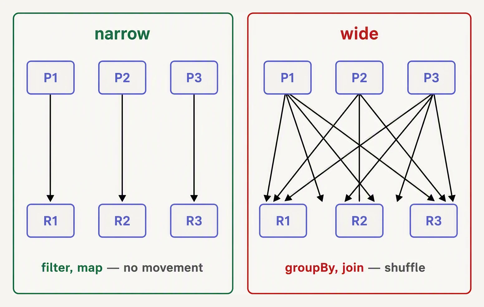
Narrow stays put. Wide crosses the network — that is the bill.
A shuffle happens when a value’s destination partition depends on a value in the data itself, not on the current partitioning.
Concrete example. You have 100 partitions of orders. You want to
groupBy("country").sum("amount"). Spark has to send every “US” row
to one executor, every “FR” row to another, etc. — across the network.
Phases of a shuffle:
- Shuffle write — each task writes per-destination files on local disk
- Network transfer — destination executors fetch those files
- Shuffle read — destination executors read the files and continue
That’s disk write + network + disk read. Each of those is 100-1000x slower than reading data already in memory. Every shuffle is a tax.
Watch rows move across the network to colocate keys
Each colored block is a row; the letter is its key. Before the shuffle, keys are scattered. Hit Shuffle to see hash partitioning: every row flies to the executor that owns its key. That flight is bytes on the wire — the network tax Spark pays every time.
The four most common shuffle triggers
| Operation | Why it shuffles |
|---|---|
groupBy(...).agg(...) | All rows with the same key must end up on one partition |
join(other, ...) (not broadcast) | Matching keys must meet on the same partition |
repartition(N) | Explicit shuffle to redistribute |
orderBy(col) (global) | Sort needs total order across all partitions |
Subtler triggers: distinct(), dropDuplicates(), window
functions (the partitionBy inside a window spec forces a shuffle),
and union followed by something that needs grouping.
You’ll spot them in the Spark UI as Exchange operators in the physical plan, and as stage boundaries with Shuffle Read / Shuffle Write metrics.
A side-by-side
# Cheap — narrow, no shuffle
orders.filter(F.col("status") == "PAID")
      .withColumn("net", F.col("amount") - F.col("discount"))

# Expensive — wide, full shuffle
orders.groupBy("country").agg(F.sum("amount"))

# Often free if Spark can broadcast small_dim — see below
fact.join(F.broadcast(small_dim), "dim_id")

# Very expensive — global sort needs to gather all data
orders.orderBy("created_at")
The first chain is narrow — each output partition depends on only one input partition, so no data moves. The second is wide — it needs every “US” row on one executor. The fourth is a global sort — the most expensive operation in Spark.
Pattern 1 — Broadcast join
When one side of a join is small enough to fit in each executor’s memory, Spark can send the whole small table to every executor. No shuffle of the big table. This is called a broadcast hash join.
# Small dim table (under ~10MB-100MB)
products = spark.read.parquet("s3://bucket/products/")

# Large fact table
orders = spark.read.parquet("s3://bucket/orders/")

# Broadcast hint — tell Spark to send 'products' to every executor
joined = orders.join(F.broadcast(products), "product_id")
The F.broadcast(...) hint tells Spark “I want this broadcast.” Without
the hint, Spark decides automatically based on
spark.sql.autoBroadcastJoinThreshold (default 10MB).
Broadcast joins are the single biggest performance win available. A 1B-row × 10K-row join with broadcast finishes in a minute. The same join with a sort-merge shuffle could take an hour.
Pattern 2 — Pre-partition before re-using
If you groupBy("user_id") once, the shuffle is unavoidable.
But if you do multiple operations all keyed on user_id, you can
pay the shuffle once and re-use:
# Bad — shuffles twice (once per groupBy)
spend  = orders.groupBy("user_id").agg(F.sum("amount").alias("spend"))
visits = events.groupBy("user_id").agg(F.count("*").alias("visits"))

# Better — partition orders/events on user_id once, then re-use
orders_p = orders.repartition("user_id")  # one shuffle
events_p = events.repartition("user_id")  # one shuffle
spend  = orders_p.groupBy("user_id").agg(F.sum("amount").alias("spend"))
visits = events_p.groupBy("user_id").agg(F.count("*").alias("visits"))
# Both DFs are already hash-partitioned on user_id — Spark can skip
# the join shuffle because matching keys are already co-located.
joined = spend.join(visits, "user_id")     # often shuffle-free now
Better still: write the data bucketed by user_id once, and
all downstream reads avoid the shuffle entirely. (Covered in the
partitioning lesson.)
Pattern 3 — Salt skewed keys
If 90% of your rows have country = "US", the shuffle puts all those
US rows on one executor. That executor’s task takes 100x longer than
any other — and the whole stage is gated on it.
The fix is salting: add a random suffix to the hot key so the load spreads:
# Salt the hot key — pretend US is split into US_0, US_1, ... US_9
salted = orders.withColumn(
    "country_salt",
    F.concat(F.col("country"), F.lit("_"),
             (F.rand() * 10).cast("int"))
)
agg = salted.groupBy("country_salt").agg(F.sum("amount").alias("amt"))
# Then aggregate again to combine the salts back into one country.
final = (agg.withColumn("country", F.regexp_extract("country_salt", r"^(.+)_\d+$", 1))
            .groupBy("country").agg(F.sum("amt").alias("amount")))
Modern Spark (3.0+) does some of this for you via Adaptive Query Execution skew join handling. But it’s not a silver bullet — for serious skew you still need salting. Covered in detail in the skew lesson.
Reading shuffle metrics in the Spark UI
Open a slow stage and look at the Summary Metrics table:
                  Min   25%   50%   75%   Max
Shuffle Read     2 MB  5 MB  6 MB  8 MB  500 MB
Task Duration    1 s   3 s   3 s   4 s   180 s
That Max column is your enemy. A Max of 500MB vs a median of 6MB means one task is doing 80x the work of others — classic skew.
The single most useful Spark UI tab is SQL → DAG → click a stage. You’ll see Exchange nodes with sizes. Anything 10x bigger than expected is suspicious.
A toy shuffle
The mechanics in 12 lines of Python:
# Toy shuffle: simulate moving rows between partitions on groupBy
import hashlib

from collections import defaultdict

# Input: 4 partitions, each with some (key, amount) rows
input_partitions = [
    [("US", 10), ("FR", 5),  ("US", 7)],
    [("DE", 3),  ("US", 12), ("FR", 4)],
    [("US", 6),  ("US", 8),  ("DE", 2)],
    [("FR", 9),  ("US", 5),  ("DE", 4)],
]

# Phase 1: each partition writes per-destination shuffle files.
# (A *deterministic* hash, so the same key always routes to the same slot.)
def dest(key, n=3):
    return int(hashlib.md5(key.encode()).hexdigest(), 16) % n

shuffle_writes = [defaultdict(list) for _ in input_partitions]
for i, part in enumerate(input_partitions):
    for k, v in part:
        shuffle_writes[i][dest(k)].append((k, v))

# Phase 2: destination partitions read everyone's files for their slot
output_partitions = defaultdict(list)
for src_writes in shuffle_writes:
    for dst, rows in src_writes.items():
        output_partitions[dst].extend(rows)

# Phase 3: aggregate within each destination
print("After shuffle, partitions hold:")
for dst in sorted(output_partitions):
    print(f"  partition {dst}: {output_partitions[dst]}")

print("\nFinal sums:")
totals = defaultdict(int)
for rows in output_partitions.values():
    for k, v in rows:
        totals[k] += v
for k, v in sorted(totals.items()):
    print(f"  {k}: {v}")
After shuffle, partitions hold:
partition 0: [('US', 10), ('FR', 5), ('US', 7), ('US', 12), ('FR', 4), ('US', 6), ('US', 8), ('FR', 9), ('US', 5)]
partition 1: [('DE', 3), ('DE', 2), ('DE', 4)]
Final sums:
DE: 9
FR: 18
US: 48That phase-1-write / phase-2-read split is exactly what Spark does —
only across a thousand machines and a real network instead of a for
loop, which is precisely why it’s the slow part.
But look harder at where the rows landed, because this tiny run accidentally demonstrates the shuffle’s nastiest failure mode. All nine US-and-FR rows hashed to partition 0, while DE’s three rows got partition 1 to themselves (and partition 2 stayed empty).
That is skew: one partition holding 9 rows next to one holding 3.
On a real cluster, the executor handed partition 0 would grind through
3× the work and gate the whole stage on itself — exactly the long-tail
task you’d hunt for in the Spark UI’s Max column.
The sums still come out right (US 48, FR 18, DE 9); they just come out slowly.
In one breath
A shuffle is when a row’s destination partition depends on the data itself (not the current layout), forcing three costly phases:
- shuffle write to local disk
- network transfer
- shuffle read
Each phase is 100–1000× slower than reading memory, which is why it dominates job cost.
The common triggers are groupBy/agg, non-broadcast join,
repartition, and global orderBy (plus distinct and windows).
The three ways to fight it are:
- broadcast join (ship a small table to every executor so the big one never moves — the single biggest win)
- pre-partition once and reuse the layout across keyed ops
- salt a hot key to break up the skew where one partition would otherwise carry everything.
Practice
Before the quiz, reach for the highest-leverage fix. You have a 1-billion-row fact table joined to a 50,000-row dimension and the job takes an hour. Name the one-line change that likely cuts it to minutes, and the exact reason it removes the shuffle.
Then connect it to the toy output above: partition 0 ended up with 9 rows and partition 1 with 3. Which of the three patterns (broadcast, pre-partition, salt) is the cure for that specific problem, and why won’t a broadcast join help it?
Quick check
A question to carry forward
That closes the architecture chapter. Step back and see what you’ve built: you know the actors that run a job, the Job→Stage→Task hierarchy they execute, why Spark defers everything until an action, and what makes the shuffle the expensive heart of it all. You understand the machine.
But notice that every example across these four lessons did the same quiet thing — it wrote:
orders.filter(...)fact.join(...)df.groupBy("country")
These examples leaned on an object we have used relentlessly and never once formally introduced: the DataFrame itself. We’ve been operating the controls of a machine while talking only about its engine.
So the question to carry forward, out of the architecture and into the next chapter, is the most basic one, the one all that machinery was built to serve.
What is a Spark DataFrame — how do you create one, what is it really (a distributed table? a plan? both?), and how is it different from the pandas DataFrame you already know?
That is the DataFrame, and it opens the next chapter — where we stop studying the engine and start driving it.
Practice this in an interview
All questionsA shuffle redistributes data across all executors so that rows with the same key end up on the same partition. It involves writing intermediate data to disk, transferring it over the network, and re-reading it — making it the most costly operation in a Spark job in terms of latency and I/O.
Data skew occurs when one or more keys concentrate disproportionately more rows than others, causing a few tasks to process gigabytes while the rest finish in seconds — one slow task stalls the entire stage. Salting appends a random suffix to skewed keys before a join or aggregation, spreading the hot key across multiple partitions, then removes the salt after aggregation.
Narrow transformations compute each output partition using data from exactly one input partition — no data moves across the network. Wide transformations require data from multiple input partitions, forcing a shuffle across the network, which is the most expensive operation in a Spark job.
repartition triggers a full shuffle to produce exactly N evenly distributed partitions and can both increase and decrease partition count. coalesce merges existing partitions on the same or nearby executors without a shuffle, but can only decrease partition count and may produce uneven partitions.