Partitioning — runtime and on disk
Two meanings of "partition" you need to keep straight. Runtime partitions split tasks across executors; storage partitions split files on disk and enable predicate pushdown.
Written and reviewed by Shreyash Prashu Last reviewed
What you'll learn
- repartition vs coalesce — when each is the right answer
- Partitioning on write —
partitionBy("date")and predicate pushdown - The 200-default-partitions trap and the small-files problem
Before you start
AQE closed the last lesson by re-tuning the query while it ran — re-counting partitions, flipping joins to broadcast, splitting stragglers. Powerful. But there was one lever even AQE couldn’t reach: how the bytes physically sit on disk before the query starts. That layout is yours to choose, not the optimizer’s, and for a large table it is the single biggest decision you make. It is called partitioning — and the word is overloaded, which is exactly where the confusion begins.
“Partition” names two distinct concepts in Spark, and they confuse everyone for their first month:
- Runtime partitions — how a DataFrame is split across executors in memory (and how many tasks run)
- Storage partitions — how files are laid out on disk (Hive-style folder hierarchy)
Both matter, but for different reasons. Get the distinction straight and the rest of this lesson clicks.
Runtime partitioning
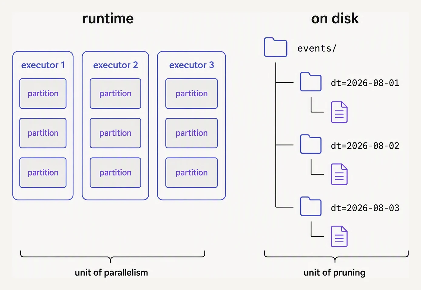
Two different things share one word: parallelism in memory, folders on disk.
In memory, a DataFrame is split into N runtime partitions. Each partition becomes one task. Each task runs on one core of one executor.
You can see the count and control it:
df.rdd.getNumPartitions()      # how many partitions right now

df.repartition(100)            # full shuffle to exactly 100 partitions
df.coalesce(50)                # combine partitions, no shuffle, may be uneven
df.repartition("country")      # hash partition by country
df.repartition(50, "country")  # 50 partitions, hashed by country
repartition vs coalesce
The most-asked-about pair in PySpark interviews:
| Operation | Shuffles? | Output balance | Use when |
|---|---|---|---|
repartition(N) | Yes (full shuffle) | Even partition sizes | You want exactly N balanced partitions |
coalesce(N) | No (combines existing) | Often uneven | You only want to reduce partition count |
Concrete: you have 1,000 partitions of ~10MB each (small-files problem incoming). You want to write 100 larger files.
# coalesce — no shuffle, combines adjacent partitions
df.coalesce(100).write.parquet("...")    # fast, but partition sizes may vary

# repartition — full shuffle, balanced output
df.repartition(100).write.parquet("...")  # slower, but every file is even
Rule of thumb: coalesce for reducing, repartition for increasing or
rebalancing. And for rebalancing on a key, repartition("user_id")
is what enables shuffle-free downstream joins.
The 200-default-partitions trap
After every shuffle, Spark targets 200 partitions by default. This is
controlled by spark.sql.shuffle.partitions, and it’s been the
default forever.
For a 10TB job, 200 partitions means each partition is 50GB — way too big, executors OOM. For a 200MB job, 200 partitions means each is 1MB — way too small, scheduling overhead dominates.
AQE largely fixes this (covered in the AQE lesson) by coalescing tiny partitions automatically. But for very large jobs where AQE hasn’t kicked in yet, set it manually:
# Tune to your data size
spark.conf.set("spark.sql.shuffle.partitions", "2000")
A rough heuristic: aim for ~128-256MB per partition.
Storage partitioning — write to folders
When you write data, you can split it into folders by a column value. This is Hive-style partitioning:
(orders.write
  .partitionBy("date")
  .parquet("s3://bucket/orders/"))
Folder layout on S3:
s3://bucket/orders/
├── date=2026-05-26/
│   ├── part-00000-....parquet
│   └── part-00001-....parquet
├── date=2026-05-27/
│   ├── part-00000-....parquet
│   └── ...
└── date=2026-05-28/
    └── ...
Now when a downstream job queries:
recent = spark.read.parquet("s3://bucket/orders/") \
              .filter(F.col("date") == "2026-05-28")
Spark notices the filter on the partition column and skips reading the other date folders entirely. This is partition pruning at scan time — often a 100-1000x reduction in I/O.
When to partition by what
Good partition columns are:
- Used in WHERE clauses often — date, region, customer_tier
- Low to medium cardinality — 10s to 1000s of distinct values
- Stable — the value doesn’t change, so old partitions stay closed
Bad partition columns:
- High cardinality — user_id with millions of values creates millions of tiny folders (small-files problem at the metadata level)
- Rarely filtered on — you pay the cost without the benefit
- Changing — you’d have to rewrite old partitions
The single most common production partitioning: date (or date_hour)
plus a region or tenant column. That covers most temporal queries.
The small-files problem
Partitioning by (date, country) looks great until you write a small
dataset:
s3://bucket/orders/date=2026-05-28/country=AF/part-00000.parquet  (4KB!)
s3://bucket/orders/date=2026-05-28/country=AL/part-00000.parquet  (8KB!)
...
Tiny files kill performance. Each file has fixed metadata cost (footer reads, listing time on S3); for 100,000 4KB files, the metadata cost dwarfs the data.
Fixes:
- Repartition before writing so each partition writes one larger file
(the
repartitionco-locates all rows for the same date+country onto one task, so each task writes one file instead of many):(df.repartition("date", "country") .write.partitionBy("date", "country").parquet("...")) - Use Delta/Iceberg and run their
OPTIMIZE/ compact operation periodically - Pick lower-cardinality partition columns — partition by
dateonly, not by(date, user_id)
Bucketing — partitioning without folders
Bucketing is a related but rarely-used feature: instead of folders per value, you put data in a fixed number of buckets based on a hash of the key:
(df.write
  .bucketBy(50, "user_id")
  .sortBy("user_id")
  .saveAsTable("orders_bucketed"))
The promise: future joins on user_id know the data is already
hash-partitioned and skip the shuffle. The reality: bucketing requires
saving to the Hive metastore, has fragile interactions with Spark
versions, and is largely replaced by Iceberg/Delta’s table-level
clustering. You’ll see it in legacy code; you’ll rarely write it new.
A toy partitioning pass
To see partition pruning concretely:
# Toy: partition pruning at scan time

# Files laid out by date
files = {
    "date=2026-05-26": ["row1", "row2"] * 1000,
    "date=2026-05-27": ["row3", "row4"] * 1000,
    "date=2026-05-28": ["row5", "row6"] * 1000,
    "date=2026-05-29": ["row7", "row8"] * 1000,
}

def scan(filter_partition=None):
    rows_read = 0
    partitions_scanned = 0
    for partition_key, rows in files.items():
        if filter_partition and partition_key != filter_partition:
            continue   # PARTITION PRUNING — skip without reading
        partitions_scanned += 1
        rows_read += len(rows)
    return rows_read, partitions_scanned

# Without pruning: scans every partition
rows, parts = scan()
print(f"No filter:        {rows:,} rows from {parts} partitions")

# With pruning: only one partition
rows, parts = scan(filter_partition="date=2026-05-28")
print(f"date=2026-05-28:  {rows:,} rows from {parts} partitions")
No filter: 8,000 rows from 4 partitions
date=2026-05-28: 2,000 rows from 1 partitionsOne filter, three folders never opened. Spark’s pruning is the same idea, applied to thousands of partitions in S3 at metadata-listing time — it lists only the folders whose names match the filter and never touches the rest.
In one breath
“Partition” means two things, and keeping them straight is the whole game.
Runtime partitions slice a DataFrame across executors in memory —
one partition, one task. You grow or rebalance them with
repartition (full shuffle, even sizes) and shrink them with
coalesce (no shuffle, possibly uneven, and watch out — it throttles
upstream parallelism too).
Storage partitions lay files into folders on disk with
partitionBy("date"), so a query that filters on that column skips
every other folder at scan time — the 100-1000x win called partition
pruning.
Pick partition columns that are low-to-medium cardinality and frequently filtered; pick wrong and you trade balanced reads for millions of tiny files.
Practice
Before the quiz, reason it through: you have a 2TB events table that
analysts almost always query as WHERE event_date = ... AND region = .... What do you partitionBy, in what order, and what would break if
you bolted on user_id as a third partition column?
Quick check
.partitionBy('date') on a frequently-filtered date column?user_id (millions of values) usually a bad idea?A question to carry forward
Everything in this lesson assumed you can spread the data evenly — pick a sensible column, get balanced folders and balanced tasks, done.
But what about data that refuses to balance? When one value —
country = "US", or a flood of NULLs in a join key — holds 80% of
the rows, no partition count saves you. Hash them however you like,
and they all pile onto a single task while the rest of the cluster sits
idle, watching.
That one overloaded task, dragging an entire stage behind it long after every sibling has finished, is the single most common production Spark failure there is. It has a name — and a toolkit of fixes. That is the next lesson.
Practice this in an interview
All questionsPartitioning divides a large table into smaller physical segments (partitions) based on a column value, so the planner can skip irrelevant partitions entirely — a technique called partition pruning. It improves performance for queries that filter on the partition key, and it simplifies bulk data management tasks like dropping old data by dropping a partition instead of issuing a slow DELETE.
repartition triggers a full shuffle to produce exactly N evenly distributed partitions and can both increase and decrease partition count. coalesce merges existing partitions on the same or nearby executors without a shuffle, but can only decrease partition count and may produce uneven partitions.
Columnar storage colocates values from the same column on disk, so aggregation queries read only the columns they need rather than full rows — dramatically reducing I/O on wide tables. Partitioning physically separates data into subdirectories (e.g., by date), allowing the query engine to skip entire partitions whose predicate cannot match, cutting scan volume from the full table to just the relevant slice.
Narrow transformations compute each output partition using data from exactly one input partition — no data moves across the network. Wide transformations require data from multiple input partitions, forcing a shuffle across the network, which is the most expensive operation in a Spark job.