Series
A Series is a 1D labeled array — the building block of every DataFrame, and the source of pandas' most magical (and most confusing) behavior.
Written and reviewed by Shreyash Prashu Last reviewed
What you'll learn
- What a Series is and how it differs from a list or ndarray
- Three ways to build one — from list, dict, and ndarray
- Why two Series with different indices align on addition (the famous gotcha)
- How the
nameattribute and the index work together
Before you start
The last lesson closed NumPy on a pointed observation: the array is fast, but anonymous — position 0, position 1, one dtype, no labels. pandas fixes exactly that, and its atom is the Series: a 1-D array that has grown an index, so every value now carries a label. That sounds like a small addition. It is not. The index is what lets you look a row up by name, what aligns two datasets that arrived in different orders, and what produces pandas’ single most magical — and most confusing — behaviour. Every column you have ever pulled out of a DataFrame was a Series.
Building a Series
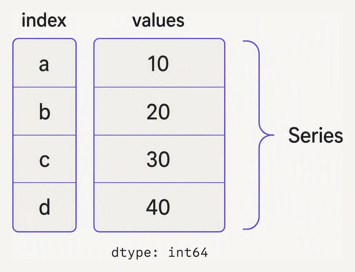
A Series is values plus an index — the index is what makes alignment automatic.
import pandas as pd
import numpy as np

# 1. From a list — index defaults to 0, 1, 2, ...
sales = pd.Series([120, 95, 140, 210, 175])
print(sales)
print()

# 2. From a dict — keys become the index
daily = pd.Series({
    "2026-05-20": 120,
    "2026-05-21":  95,
    "2026-05-22": 140,
    "2026-05-23": 210,
    "2026-05-24": 175,
}, name="units_sold")
print(daily)
print()

# 3. From a NumPy ndarray, with a custom index
prices = pd.Series(np.array([19.99, 24.99, 9.99]),
                   index=["pen", "notebook", "eraser"],
                   name="price_usd")
print(prices)
0 120
1 95
2 140
3 210
4 175
dtype: int64
2026-05-20 120
2026-05-21 95
2026-05-22 140
2026-05-23 210
2026-05-24 175
Name: units_sold, dtype: int64
pen 19.99
notebook 24.99
eraser 9.99
Name: price_usd, dtype: float64Three constructions, three indices: the list got a default 0…4, the dict turned its keys into the
labels, and the ndarray took a custom index. The name attribute becomes the column name when
this Series is joined into a DataFrame — set it early, it pays off later.
The index is the secret sauce
Unlike a Python list, a Series looks values up by their label:
import pandas as pd

prices = pd.Series(
    [19.99, 24.99, 9.99, 4.50],
    index=["pen", "notebook", "eraser", "stapler"],
    name="price_usd",
)

print(prices["notebook"])        # 24.99 — by label
print(prices.iloc[0])             # 19.99 — by integer position
print(prices[["pen", "eraser"]])  # multiple labels at once

# The two parts
print("\nvalues:", prices.values)   # the underlying numpy array
print("index:", prices.index)        # the labels
print("name:", prices.name)
24.99
19.99
pen 19.99
eraser 9.99
Name: price_usd, dtype: float64
values: [19.99 24.99 9.99 4.5 ]
index: Index(['pen', 'notebook', 'eraser', 'stapler'], dtype='object')
name: price_usdKeep three things in mind about every Series: values (the underlying NumPy array — pandas really
is NumPy with labels bolted on), index (the labels), and name (what it will be called as a
DataFrame column). ["notebook"] looked up by label, .iloc[0] by position — both routes, side by
side.
Alignment — the magic, and the gotcha
This is the single biggest “huh?” moment in pandas. When you add two Series, pandas aligns them by index label, not by position:
import pandas as pd

# Sales by product, store A and store B
store_a = pd.Series(
    {"pen": 120, "notebook": 95,  "eraser": 40},
    name="units",
)

store_b = pd.Series(
    {"notebook": 80, "pen": 110, "stapler": 12},
    name="units",
)

# Surprise: not [200, 175, ...] — pandas matches by label
total = store_a + store_b
print(total)
eraser NaN
notebook 175.0
pen 230.0
stapler NaN
Name: units, dtype: float64Read the result carefully — two things happened:
pen(120 + 110 = 230) andnotebook(95 + 80 = 175) added correctly even though they appear in different orders in the two Series. Pandas matched them by label, not position.eraser(only in A) andstapler(only in B) became NaN — pandas’ floating-point sentinel for “missing” — because there was nothing on the other side to add.
If you want the lonely keys filled with zero instead of NaN, use .add() with fill_value:
import pandas as pd

store_a = pd.Series({"pen": 120, "notebook": 95, "eraser": 40})
store_b = pd.Series({"notebook": 80, "pen": 110, "stapler": 12})

total = store_a.add(store_b, fill_value=0)
print(total)
eraser 40.0
notebook 175.0
pen 230.0
stapler 12.0
dtype: float64Now eraser keeps its 40 and stapler its 12 — the missing side is treated as 0 rather than
poisoning the result with NaN.
Series operations are vectorized
Vectorized means the operation runs over every element at once — no Python for loop — because
pandas hands the work to compiled C/NumPy underneath (the why-numpy story, one
layer up). Arithmetic, comparison, and method calls all run over the whole array:
import pandas as pd

prices = pd.Series(
    [19.99, 24.99, 9.99, 4.50],
    index=["pen", "notebook", "eraser", "stapler"],
)

print(prices * 1.08)              # add 8% tax
print()
print(prices > 10)                # boolean Series
print()
print(prices[prices > 10])        # boolean indexing
print()
print(prices.describe())          # summary stats
pen 21.5892
notebook 26.9892
eraser 10.7892
stapler 4.8600
dtype: float64
pen True
notebook True
eraser False
stapler False
dtype: bool
pen 19.99
notebook 24.99
dtype: float64
count 4.000000
mean 14.867500
std 9.309137
min 4.500000
25% 8.617500
50% 14.990000
75% 21.240000
max 24.990000
dtype: float64prices * 1.08 taxed all four at once; prices > 10 returned a boolean Series; prices[prices > 10] is the NumPy boolean-mask idiom, now carrying labels; and .describe() is the one-call summary
you will reach for on every new column. Every one of these keeps the index — the labels ride along.
In one breath
A Series is a 1-D NumPy array plus an index (a label on every value), with three parts:
values (the ndarray), index (the labels), name (its future DataFrame column). Build one
from a list (default 0…n index), a dict (keys → index), or an ndarray (custom index). Look up by
label (s["notebook"]) or position (s.iloc[0]). The headline behaviour — and the famous
gotcha — is automatic alignment: arithmetic between two Series matches by label, not
position, so mismatched labels yield NaN (use .add(other, fill_value=0) to fill instead).
Operations are vectorized and keep the index, so prices * 1.08, prices > 10, masks, and
.describe() all carry their labels along.
Practice
Quick check
pd.Series({'a': 1, 'b': 2}) + pd.Series({'b': 10, 'c': 20})?s = pd.Series([10, 20, 30], index=['x', 'y', 'z']), what does s.iloc[0] return?prices_jan (index ['a','b','c']) and prices_feb (index ['b','c','d']). How many NaN values are in the result?A question to carry forward
A Series is one labeled column. But real data never arrives as a lone column — it comes as a
table: many columns, often of different types (a string name, a float price, an int
quantity), all sharing one index and sitting side by side. Stack a pile of Series that share an
index and you have the object pandas is really built around: the DataFrame.
So the next lesson opens it up. What is a DataFrame — a dict of Series glued to one common index — how do you build one, inspect its shape and dtypes, and reach into its rows and columns? And here is the thread to hold onto: the label-alignment you just met on a single Series is the same machinery that will line up entire tables when you start joining them.
Practice this in an interview
All questionsBoolean indexing filters a DataFrame by passing a boolean Series or array of the same length as the index. Common pitfalls include using Python's and/or instead of &/| and forgetting to wrap compound conditions in parentheses, both of which raise errors or produce wrong results.
concat stacks DataFrames along an axis without matching keys; join aligns on the index (or a single key column) using a convenient shorthand; merge is the most general, joining on any column(s) with full SQL-style control over the join type, key names, and suffix handling.
Wide format stores multiple measurements as separate columns per subject; long (tidy) format stores one measurement per row with a variable-name column and a value column. Long format is required by most statistical and visualization libraries, makes adding new variables trivial, and is the standard expected by groupby and merge operations.
CategoricalDtype stores a column as integer codes plus a small lookup table of unique values, dramatically reducing memory for low-cardinality string columns. It also enforces a fixed set of valid values, enables natural ordering, and speeds up groupby and sort operations.