Reshape — pivot, melt, stack, unstack
Turn long event logs into wide feature tables and back. The four verbs that move data between "tidy" and "human-readable" shapes.
Written and reviewed by Shreyash Prashu Last reviewed
What you'll learn
- The difference between long and wide formats — and when each is right
-
pivotvspivot_tableand the duplicate-key gotcha -
melt— the inverse of pivot -
stackandunstackfor multi-index data
Before you start
The last lesson handed you the third axis of data manipulation it promised: not joining two tables, but reshaping a single one. Data lives in two shapes — long (one row per observation, easy to log and aggregate) and wide (one row per entity, easy to read or feed to a model).
Real jobs make you move between them constantly: pivot a tidy event log into per-user features, or melt a wide quarterly report into something you can plot. Four verbs do almost all of it.
Long vs wide — a concrete example
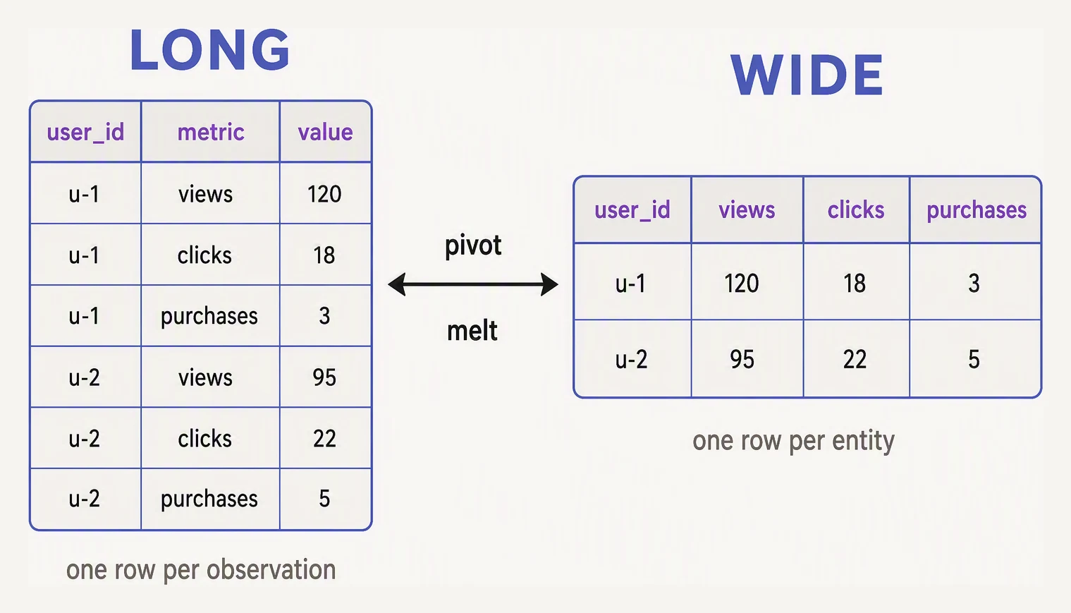
pivot goes long to wide. melt goes back.
import pandas as pd

# LONG: one row per (user, metric) observation
long = pd.DataFrame({
    "user_id": ["u-1","u-1","u-1","u-2","u-2","u-2","u-3","u-3"],
    "metric":  ["views","clicks","purchases","views","clicks","purchases","views","clicks"],
    "value":   [120, 18, 3, 95, 22, 5, 60, 7],
})
print("LONG:")
print(long)
print()

# WIDE: one row per user, one column per metric
wide = long.pivot(index="user_id", columns="metric", values="value")
print("WIDE:")
print(wide)
LONG:
user_id metric value
0 u-1 views 120
1 u-1 clicks 18
2 u-1 purchases 3
3 u-2 views 95
4 u-2 clicks 22
5 u-2 purchases 5
6 u-3 views 60
7 u-3 clicks 7
WIDE:
metric clicks purchases views
user_id
u-1 18.0 3.0 120.0
u-2 22.0 5.0 95.0
u-3 7.0 NaN 60.0Long format is what databases naturally produce: one row per event, per (user, day, metric) tuple. Wide is what humans read in reports and what most ML libraries expect as a feature matrix.
Note u-3 made no purchases, so its purchases cell came back NaN — the gap a missing observation
leaves when you spread a column out.
pivot — long to wide (no aggregation)
pivot(index, columns, values) works only when each (index, columns) pair appears exactly once.
It is a pure reshape with no aggregation step.
If two rows land in the same cell, pivot cannot decide which value goes there. It errors out rather than silently picking one:
import pandas as pd

# Same metric for same user shows up twice (e.g. two days of data) → duplicates
events = pd.DataFrame({
    "user_id": ["u-1","u-1","u-1","u-1"],
    "metric":  ["views","views","clicks","clicks"],
    "value":   [120, 30, 18, 5],
})

try:
    events.pivot(index="user_id", columns="metric", values="value")
except ValueError as e:
    print("pivot error:", e)
pivot error: Index contains duplicate entries, cannot reshapeThat error is pivot protecting you — u-1 has two views rows (120 and 30), and pivot refuses to
guess. When you have duplicates and genuinely need to combine them, reach for pivot_table.
pivot_table — long to wide with aggregation
pivot_table is pivot + groupby. It collapses duplicates using an aggregation function (default:
mean):
import pandas as pd

events = pd.DataFrame({
    "user_id": ["u-1","u-1","u-1","u-1","u-2","u-2"],
    "metric":  ["views","views","clicks","clicks","views","clicks"],
    "value":   [120, 30, 18, 5, 95, 22],
})

# Sum metric values per user
wide_sum = events.pivot_table(
    index="user_id",
    columns="metric",
    values="value",
    aggfunc="sum",
    fill_value=0,
)
print(wide_sum)
print()

# You can have multiple aggregations
wide_multi = events.pivot_table(
    index="user_id",
    columns="metric",
    values="value",
    aggfunc=["sum","mean"],
).round(2)
print(wide_multi)
metric clicks views
user_id
u-1 23 150
u-2 22 95
sum mean
metric clicks views clicks views
user_id
u-1 23 150 11.5 75.0
u-2 22 95 22.0 95.0u-1’s two views (120 + 30) summed to 150 and two clicks (18 + 5) to 23. Those are the duplicates
pivot refused, aggregated on purpose.
fill_value=0 is almost always what you want for events (a user with no clicks should read 0, not
NaN), and aggfunc=["sum","mean"] stacks both stats into a two-level column header.
melt — wide to long
melt is the inverse: wide back to long, perfect for plotting libraries that want one row per data
point.
import pandas as pd

# Wide quarterly report — typical from finance teams
report = pd.DataFrame({
    "product":  ["Pen", "Notebook", "Eraser"],
    "Q1_2026":  [12000, 8000, 3000],
    "Q2_2026":  [13500, 8400, 2800],
    "Q3_2026":  [14200, 9000, 3100],
    "Q4_2026":  [15000, 9500, 3300],
})
print("WIDE:")
print(report)
print()

# Melt into long form
long_report = report.melt(
    id_vars="product",
    var_name="quarter",
    value_name="revenue",
)
print("LONG (ready for plotting / SQL / groupby):")
print(long_report.head(8))
WIDE:
product Q1_2026 Q2_2026 Q3_2026 Q4_2026
0 Pen 12000 13500 14200 15000
1 Notebook 8000 8400 9000 9500
2 Eraser 3000 2800 3100 3300
LONG (ready for plotting / SQL / groupby):
product quarter revenue
0 Pen Q1_2026 12000
1 Notebook Q1_2026 8000
2 Eraser Q1_2026 3000
3 Pen Q2_2026 13500
4 Notebook Q2_2026 8400
5 Eraser Q2_2026 2800
6 Pen Q3_2026 14200
7 Notebook Q3_2026 9000The four quarter columns became rows of a single quarter column. id_vars are the columns you
keep as identifiers (product); everything else is unpivoted, with var_name/value_name naming
the resulting label and value columns.
The same data, two shapes
Long format stores one observation per row. Pivot reshapes it wide so each category becomes a column. Melt is the exact inverse — no data is created or destroyed, only the layout changes.
| date | city | metric | value |
|---|---|---|---|
| 2024-01-01 | Mumbai | sales_k | 42 |
| 2024-01-01 | Delhi | sales_k | 58 |
| 2024-01-02 | Mumbai | sales_k | 45 |
| 2024-01-02 | Delhi | sales_k | 61 |
| 2024-01-03 | Mumbai | sales_k | 39 |
| 2024-01-03 | Delhi | sales_k | 53 |
| 2024-01-04 | Mumbai | sales_k | 47 |
| 2024-01-04 | Delhi | sales_k | 66 |
df.melt(
    id_vars=["date", "metric"],
    value_vars=["Mumbai", "Delhi"],
    var_name="city",
    value_name="value",
)city column. Every value cell becomes its own row — the exact inverse of pivot.stack and unstack — for multi-index data
When you group by several columns you end up with a MultiIndex. stack and unstack move levels
between the row and column axes:
import pandas as pd

events = pd.DataFrame({
    "user_id": ["u-1","u-1","u-2","u-2","u-3","u-3"],
    "country": ["IN","IN","US","US","SG","SG"],
    "metric":  ["views","clicks","views","clicks","views","clicks"],
    "value":   [120, 18, 95, 22, 60, 7],
})

# Group by all three; result has a 3-level MultiIndex
g = events.groupby(["country","user_id","metric"])["value"].sum()
print("Grouped (MultiIndex Series):")
print(g)
print()

# Unstack: move the innermost level into columns → DataFrame
print("After unstack():")
print(g.unstack())
print()

# Unstack a specific level
print("After unstack('country') — country becomes the column axis:")
print(g.unstack("country"))
Grouped (MultiIndex Series):
country user_id metric
IN u-1 clicks 18
views 120
SG u-3 clicks 7
views 60
US u-2 clicks 22
views 95
Name: value, dtype: int64
After unstack():
metric clicks views
country user_id
IN u-1 18 120
SG u-3 7 60
US u-2 22 95
After unstack('country') — country becomes the column axis:
country IN SG US
user_id metric
u-1 clicks 18.0 NaN NaN
views 120.0 NaN NaN
u-2 clicks NaN NaN 22.0
views NaN NaN 95.0
u-3 clicks NaN 7.0 NaN
views NaN 60.0 NaNThe mental model: unstack moves a level from the row index up into the columns. Plain
unstack() took the innermost metric; unstack("country") took a named level, spreading the three
countries into columns and leaving NaN where a user has no row for that country.
stack does the reverse — pulls a column level down into the row index. Together they are the
Swiss-army knife of MultiIndex reshaping.
When wide, when long?
- Long is right for: storing data, logging events, SQL tables, plotting libraries (matplotlib/seaborn/plotly long-form), aggregating with groupby.
- Wide is right for: human-readable reports, dashboards, ML feature matrices (one row per training example), correlation matrices.
The real answer is often long → groupby/agg → wide. Don’t be afraid to round-trip.
A complete worked example — event log to ML features
import pandas as pd

# Raw event log — what your warehouse gives you (long)
events = pd.DataFrame({
    "user_id": ["u-1","u-1","u-1","u-2","u-2","u-3","u-3","u-3","u-3"],
    "event":   ["view","click","purchase","view","view","view","click","click","purchase"],
    "value":   [1, 1, 49.99, 1, 1, 1, 1, 1, 14.50],
})

# Step 1: aggregate per (user, event) — long but deduped
per_user_event = events.groupby(["user_id","event"]).agg(
    count    = ("value", "size"),
    total    = ("value", "sum"),
).reset_index()
print("Aggregated (still long):")
print(per_user_event)
print()

# Step 2: pivot to wide — one row per user, one column per event type
features = per_user_event.pivot_table(
    index="user_id",
    columns="event",
    values="count",
    fill_value=0,
).rename_axis(columns=None)              # drop the "event" name on the column axis

# Add a revenue feature
revenue = events[events["event"] == "purchase"].groupby("user_id")["value"].sum()
features["revenue"] = revenue.reindex(features.index).fillna(0).round(2)

print("ML feature table (wide, one row per user):")
print(features)
Aggregated (still long):
user_id event count total
0 u-1 click 1 1.00
1 u-1 purchase 1 49.99
2 u-1 view 1 1.00
3 u-2 view 2 2.00
4 u-3 click 2 2.00
5 u-3 purchase 1 14.50
6 u-3 view 1 1.00
ML feature table (wide, one row per user):
click purchase view revenue
user_id
u-1 1.0 1.0 1.0 49.99
u-2 0.0 0.0 2.0 0.00
u-3 2.0 1.0 1.0 14.50Long event log → group → pivot to wide → graft on a revenue column: one row per user, ready for a model. (u-2, all views and no purchases, correctly reads 0 across the board with 0 revenue.) This “events to features” pattern is something nearly every ML pipeline over a transactional system does.
In one breath
Data is long (one row per observation — log/aggregate/plot) or wide (one row per entity — read/model).
pivot(index, columns, values) spreads long → wide but errors on duplicate pairs.
pivot_table is pivot + groupby, collapsing duplicates with aggfunc (default mean,
fill_value=0 for events). Check .duplicated().any() before assuming uniqueness.
melt is the inverse (wide → long: id_vars stay, the rest unpivot into
var_name/value_name). unstack lifts a row-index level into columns and stack pushes a
column level down — the MultiIndex pair.
The everyday pipeline is long → groupby/agg → pivot-to-wide (events → ML features).
Practice
Quick check
pivot and pivot_table?df with columns ['product', 'Jan', 'Feb', 'Mar']. How do you melt it into long form?df.groupby(['country','metric']).sum(), you get a Series with a 2-level MultiIndex. How do you turn metric into columns?['respondent_id', 'age', 'q1_score', 'q2_score', 'q3_score']. You want to compute the average score across all questions using groupby. What shape transformation should you do first?A question to carry forward
You now hold the full mechanical toolkit — build, read, select, clean, group, merge, reshape — enough for the vast majority of data work. But one dimension has been quietly hiding in nearly every example: time.
We pivoted on a quarter, grouped by a day, sorted event logs by a ts — always treating the
timestamp as just another column of strings.
It is not. Time has order, a frequency, gaps, and a whole calendar. You can bucket it into days,
roll a 7-day average across it, or slice it by '2026-01' — none of which works while your dates are
mere strings.
The next lesson gives time first-class treatment: the DatetimeIndex, resample, and
rolling windows. How do you turn a string column into a real time index, and why does that one
change collapse daily rollups and moving averages into one-liners?
Practice this in an interview
All questionspivot reshapes long-format data to wide by spreading a column's values into new column headers — it requires unique index/column combinations and has no aggregation. pivottable is the aggregating version that handles duplicates via a specified aggfunc. melt is the inverse: it takes wide-format data and collapses multiple columns into key-value rows (long format).
Wide format stores multiple measurements as separate columns per subject; long (tidy) format stores one measurement per row with a variable-name column and a value column. Long format is required by most statistical and visualization libraries, makes adding new variables trivial, and is the standard expected by groupby and merge operations.
Grouping on multiple keys produces a MultiIndex on the result by default. You can suppress it with asindex=False or groupby(..., asindex=False), or reset it afterward with resetindex(). Stacking and unstacking let you pivot between long and wide forms once a MultiIndex exists.
concat stacks DataFrames along an axis without matching keys; join aligns on the index (or a single key column) using a convenient shorthand; merge is the most general, joining on any column(s) with full SQL-style control over the join type, key names, and suffix handling.