DataFrame basics
The single most important class in the Python data stack. Create one, inspect it, and select from it without surprises.
Written and reviewed by Shreyash Prashu Last reviewed
What you'll learn
- Three reliable ways to construct a DataFrame
- How to inspect a DataFrame in a few seconds
- Why
[]vs.locvs.ilocmatters
Before you start
The last lesson built a single labeled column — a Series — and promised that stacking many of them,
all sharing one index, gives the object pandas is genuinely built around: the DataFrame. Here it
is. A DataFrame is a 2-D labeled table — think spreadsheet, think SQL result set — with row
labels (the index, assigned 0, 1, 2… automatically unless you set your own) and column
labels (the columns), where each column is a Series carrying its own dtype (int64,
float64, object for strings). Everything you learned about a Series — values, index,
label-alignment — still holds, because a DataFrame is just a dict of Series glued to one shared
index.
Three ways to construct one
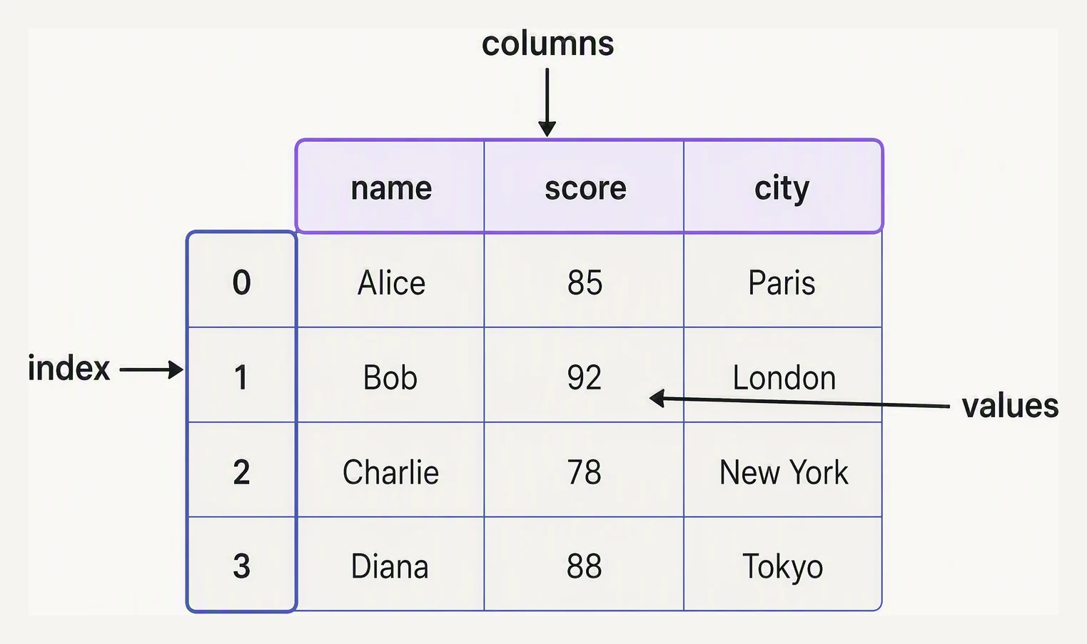
Three parts, always: an index, columns, and the values between them.
import pandas as pd

# 1. From a dict of lists — each key is a column
df1 = pd.DataFrame({
    "name":  ["Aarav", "Bea", "Chen"],
    "age":   [28, 34, 25],
    "city":  ["Mumbai", "NYC", "Beijing"],
})

# 2. From a list of dicts — each dict is a row (great when data comes from JSON)
rows = [
    {"name": "Aarav", "age": 28, "city": "Mumbai"},
    {"name": "Bea",   "age": 34, "city": "NYC"},
    {"name": "Chen",  "age": 25, "city": "Beijing"},
]
df2 = pd.DataFrame(rows)

# 3. From a CSV / Parquet file (most common in real work)
# df = pd.read_csv("path/to/data.csv")

print(df1)
name age city
0 Aarav 28 Mumbai
1 Bea 34 NYC
2 Chen 25 BeijingThe dict-of-lists reads column-wise, the list-of-dicts row-wise (perfect for JSON) — both produce
the identical table with a default 0, 1, 2 index. In a real job you will almost always use option
3 (read from a file, the next lesson); options 1 and 2 are for tests and small examples.
Inspect a DataFrame in 10 seconds
import pandas as pd

df = pd.DataFrame({
    "name":  ["Aarav", "Bea", "Chen", "Dara", "Eli"],
    "age":   [28, 34, 25, 41, 29],
    "city":  ["Mumbai", "NYC", "Beijing", "Mumbai", "NYC"],
    "salary":[55000, 92000, 48000, 110000, 75000],
})

print("--- head ---")
print(df.head(3))                # first 3 rows

print("\n--- shape ---")
print(df.shape)                  # (rows, cols)

print("\n--- dtypes ---")
print(df.dtypes)                 # one type per column

print("\n--- describe ---")
print(df.describe())             # numeric summary

print("\n--- value_counts (city) ---")
print(df["city"].value_counts())
--- head ---
name age city salary
0 Aarav 28 Mumbai 55000
1 Bea 34 NYC 92000
2 Chen 25 Beijing 48000
--- shape ---
(5, 4)
--- dtypes ---
name object
age int64
city object
salary int64
dtype: object
--- describe ---
age salary
count 5.000000 5.000000
mean 31.400000 76000.000000
std 6.268971 25680.732077
min 25.000000 48000.000000
25% 28.000000 55000.000000
50% 29.000000 75000.000000
75% 34.000000 92000.000000
max 41.000000 110000.000000
--- value_counts (city) ---
city
Mumbai 2
NYC 2
Beijing 1
Name: count, dtype: int64.head(), .shape, .dtypes, .describe(), and .value_counts() are the five calls you will run
within seconds of loading any new dataset — note describe() quietly skipped the string columns
and summarised only the numerics. Burn them into muscle memory.
Selecting columns
df["age"]            # one column → returns a Series
df[["age", "city"]]  # multiple columns → returns a DataFrame
One bracketed name gives back a Series (a single labeled column, from last lesson); a list of names gives back a smaller DataFrame. A DataFrame is, after all, just a collection of Series sharing an index.
Selecting rows — .loc vs .iloc
This is the most common source of confusion for newcomers, and the rule is genuinely simple:
.locuses labels (index values, column names). Think “loc = label.”.ilocuses integer positions (0-based). Think “iloc = integer position.”
Why does it matter? If your index is ["a", "b", "c"], df.loc["b"] fetches the row labeled "b"
wherever it sits; df.iloc[1] always fetches the second row by position, whatever its label. With
the default 0, 1, 2… index the two happen to agree — which is exactly what lulls beginners into
thinking they are interchangeable.
import pandas as pd

df = pd.DataFrame({
    "age":  [28, 34, 25, 41, 29],
    "city": ["Mumbai", "NYC", "Beijing", "Mumbai", "NYC"],
}, index=["a", "b", "c", "d", "e"])

# Label-based: rows by index label
print(df.loc["b"])
print("---")
print(df.loc[["a", "c"], "age"])

# Position-based: row 1 (the second row), column 0
print("---")
print(df.iloc[1, 0])
age 34
city NYC
Name: b, dtype: object
---
a 28
c 25
Name: age, dtype: int64
---
34df.loc["b"] returned the whole b row as a Series; df.iloc[1, 0] returned the single value at
position (row 1, col 0) — which is 34, the same number df.loc["b", "age"] would give. Same
value, two completely different addressing schemes.
Boolean filtering — the workhorse
import pandas as pd

df = pd.DataFrame({
    "name":  ["Aarav", "Bea", "Chen", "Dara", "Eli"],
    "age":   [28, 34, 25, 41, 29],
    "city":  ["Mumbai", "NYC", "Beijing", "Mumbai", "NYC"],
    "salary":[55000, 92000, 48000, 110000, 75000],
})

# Anyone over 30
print(df[df["age"] > 30])

# Anyone in NYC making over 80k — combine with & (and), | (or). Use parens!
print(df[(df["city"] == "NYC") & (df["salary"] > 80000)])
name age city salary
1 Bea 34 NYC 92000
3 Dara 41 Mumbai 110000
name age city salary
1 Bea 34 NYC 92000This is the NumPy boolean-mask idiom from the last section, now operating on whole rows of a table:
the mask df["age"] > 30 keeps Bea and Dara; combining two masks with & narrows to just Bea. The
parentheses around each comparison are required — & binds tighter than >/==, the same trap
the boolean-masks lesson warned about.
Creating, modifying, dropping columns
df["bonus"] = df["salary"] * 0.10        # new column
df["age"] = df["age"] + 1                 # modify in place
df = df.drop(columns=["bonus"])           # drop returns a new DataFrame — original unchanged
df = df.rename(columns={"city": "loc"})   # rename
In one breath
A DataFrame is a 2-D labeled table — a dict of Series sharing one index, each column its own
dtype. Build it from a dict-of-lists (column-wise), a list-of-dicts (row-wise, JSON-friendly),
or a file. Inspect any new dataset in seconds with .head() / .shape / .dtypes /
.describe() (numerics only) / .value_counts(). Select columns with df["col"] (→ Series)
or df[["a","b"]] (→ DataFrame); select rows with .loc (by label) versus .iloc (by
integer position) — they coincide only under the default integer index. Filter rows with boolean
masks (df[df["age"] > 30]), combining conditions with &/| and parenthesising each. And
never chain indexing for assignment — use a single df.loc[mask, "col"] = val.
Practice
Quick check
df?df.describe() show by default?['p', 'q', 'r']. You write df.loc['q':'r', 'age']. How many rows are returned?A question to carry forward
Every DataFrame in this lesson was hand-built from a dict or a list — perfect for examples, but in a real job you will almost never type your data in. It arrives in a file: a comma- or semicolon-separated CSV with comment lines stapled to the top, a binary Parquet, a line-delimited JSON, a SQL table behind a connection.
So the next lesson is the doorway every data project actually starts at — pd.read_csv and its
cousins, very likely the most-called function in the whole Python data stack. Which of its dozen
arguments turn a “this won’t parse” export into a clean, correctly-typed DataFrame; when should you
reach for Parquet over CSV; and how do you read a file that is bigger than your RAM?
Practice this in an interview
All questionsConvert string columns to datetime with pd.todatetime(), then use the .dt accessor to extract components like year, month, day, and day of week, compute time deltas, and perform resampling. Setting a DatetimeIndex unlocks time-series-specific operations like resample, rolling, and time-aware interpolation.
duplicated() returns a boolean mask of rows that are duplicates of an earlier row; dropduplicates() removes them. Both accept a subset parameter to restrict comparison to specific columns and a keep parameter ('first', 'last', or False) to control which instance is retained or whether all copies are dropped.
pandas is slow primarily because Python loops bypass NumPy's vectorized C kernels, object-dtype columns prevent SIMD optimizations, and keeping entire datasets in memory limits scalability. The fixes are vectorization, categorical encoding, eval/query for large frames, chunking for out-of-core data, and switching to Polars or DuckDB for compute-heavy pipelines.
concat stacks DataFrames along an axis without matching keys; join aligns on the index (or a single key column) using a convenient shorthand; merge is the most general, joining on any column(s) with full SQL-style control over the join type, key names, and suffix handling.