Reading data
read_csv, read_parquet, read_json, read_sql — and the half-dozen arguments that turn a "this won't parse" file into a clean DataFrame.
Written and reviewed by Shreyash Prashu Last reviewed
What you'll learn
- The most-used
read_csvarguments and when to reach for each - How to skip junk rows in a messy real-world CSV
- When to use Parquet over CSV (almost always, for large data)
- How to write data back out — and which format to choose
Before you start
The last lesson built DataFrames by hand from dicts and lists. Real data never arrives that way — it comes in a file.
pd.read_csv is very likely the most-called function in the entire Python data ecosystem. In a real
job you will spend more time wrangling its arguments than writing any other line of pandas. This
lesson is why: the handful of arguments that turn a malformed, comment-strewn, semicolon-delimited
export into a clean, correctly-typed DataFrame.
The minimal call
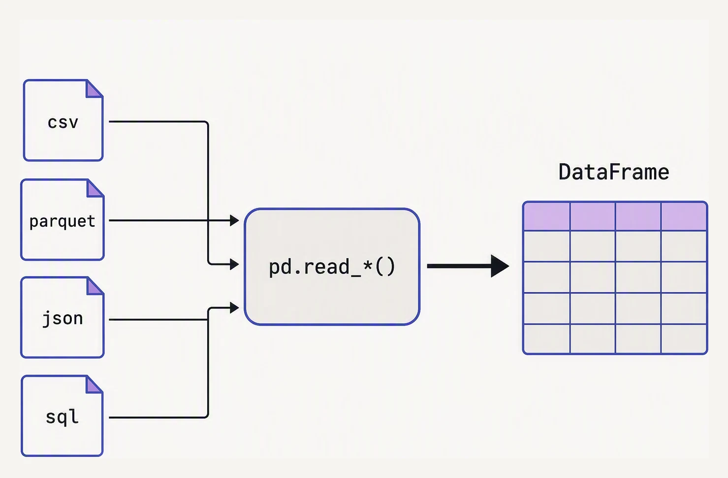
Different doors, same room — every reader lands you in a DataFrame.
import pandas as pd

df = pd.read_csv("orders.csv")
That works on perfectly formatted files. Real files are not perfectly formatted.
The arguments you’ll actually use
import pandas as pd

from io import StringIO

raw = """# Orders export from CRM, generated 2026-05-27
# DO NOT EDIT
order_id;customer_id;order_date;amount_usd;notes
1001;C-22;2026-05-01;129.50;rush
1002;C-15;2026-05-01;85.00;
1003;C-22;2026-05-02;212.00;gift wrap
1004;C-09;2026-05-02;47.25;
"""

df = pd.read_csv(
    StringIO(raw),
    sep=";",                        # this file uses ; not ,
    skiprows=2,                     # skip the two comment lines
    parse_dates=["order_date"],     # parse as datetime
    dtype={"customer_id": "string", "notes": "string"},
    usecols=["order_id", "customer_id", "order_date", "amount_usd"],
)
print(df)
print()
print(df.dtypes)
order_id customer_id order_date amount_usd
0 1001 C-22 2026-05-01 129.50
1 1002 C-15 2026-05-01 85.00
2 1003 C-22 2026-05-02 212.00
3 1004 C-09 2026-05-02 47.25
order_id int64
customer_id string[python]
order_date datetime64[ns]
amount_usd float64
dtype: objectFive arguments turned a semicolon-delimited file with two comment lines into a clean frame.
order_date came back as a real datetime64, customer_id as a proper string, and the notes
column was dropped by usecols.
The arguments worth knowing by heart:
sep— column separator. Default is,. European exports often use;. TSVs use\t.header— row index of the column names. Setheader=Noneif the file has no header (and passnames=[...]to provide them).names— explicit column names (use withheader=Noneor to override).skiprows— drop the first N rows of garbage, or pass a list of row indices.dtype— force specific column types. Stops pandas from inferring strings as floats, IDs as ints, etc.parse_dates— list of columns to parse as datetime. Saves apd.to_datetimestep later.usecols— only read these columns. Faster, less memory.nrows— read just the first N rows. Perfect when prototyping against a 50 GB file.chunksize— instead of reading the whole file at once, return an iterator of DataFrames, N rows each. Use it when the file is bigger than RAM.
Skipping junk rows (the real-world CSV)
You will get a CSV from an enterprise system that looks like this — comments at the top, a blank line, then the real data:
import pandas as pd

from io import StringIO

raw = """Sales Report
Generated by FinanceBot v3.2
Period: 2026-Q2

product,quantity,price
"Pen",120,1.99
"Notebook",85,4.50
"Eraser",40,0.75
"""

df = pd.read_csv(StringIO(raw), skiprows=4)
print(df)
product quantity price
0 Pen 120 1.99
1 Notebook 85 4.50
2 Eraser 40 0.75Three lines of header garbage plus one blank line — skiprows=4 lands you exactly on the real header
row. If the junk lines vary in count, pass a callable instead: skiprows=lambda i: i < 4.
Reading big files in chunks
import pandas as pd

from io import StringIO

raw = "user_id,event\n"
for i in range(20):
    raw += f"u{i % 4},click\n"

# Pretend this is a 50 GB file — read 5 rows at a time
total_by_user = pd.Series(dtype=int)
for chunk in pd.read_csv(StringIO(raw), chunksize=5):
    counts = chunk["user_id"].value_counts()
    total_by_user = total_by_user.add(counts, fill_value=0)

print(total_by_user.astype(int))
user_id
u0 5
u1 5
u2 5
u3 5
dtype: int64chunksize is your way out when the file does not fit in memory. Process one chunk at a time and
aggregate as you go.
Here the 20 rows arrived in four chunks of five. The per-chunk value_counts were summed with the
.add(..., fill_value=0) alignment trick from the Series lesson — five clicks for each of the
four users.
Parquet — your new default for large data
CSV is text. Every read has to re-parse, re-type, and re-decode strings. Parquet is a binary, columnar format that is typically 5–10× smaller and 10–100× faster to read:
df.to_parquet("orders.parquet")          # write
df = pd.read_parquet("orders.parquet") # read — types preserved, no parse_dates neededJSON and SQL
# JSON: line-delimited (one record per line) is the common case
df = pd.read_json("events.jsonl", lines=True)

# SQL: pass a connection (sqlite3, SQLAlchemy, etc.)
import sqlite3

con = sqlite3.connect("warehouse.db")
df = pd.read_sql("SELECT * FROM orders WHERE order_date >= '2026-05-01'", con)
For SQL, push filtering and aggregation into the database whenever you can. Don’t pull a 100M-row table into pandas if you only need a sum.
Writing data back out
df.to_csv("out.csv", index=False)        # index=False = don't write the row index as a column
df.to_parquet("out.parquet")              # binary, compact, fast
df.to_json("out.jsonl", orient="records", lines=True)
df.to_sql("orders", con, if_exists="append", index=False)
index=False on to_csv saves you from the dreaded “Unnamed: 0” column reappearing next time
someone re-reads the file. Almost always what you want.
In one breath
pd.read_csv is the doorway to most data work, and a few arguments tame any messy export:
sep(;/\t)skiprows(drop comment lines, or alambda)header/names(no/own headers)dtype(force types)parse_dates(realdatetime64)usecols(fewer columns, less memory)nrows(prototype on a slice)chunksize(iterate a larger-than-RAM file, aggregating per chunk)
For anything large or re-read, switch to Parquet — binary, columnar, type-preserving, 5–10×
smaller and far faster than CSV. Read JSON with read_json(lines=True) and SQL with read_sql
(push filtering into the DB). Write back with to_csv(index=False), to_parquet, to_json,
to_sql.
Practice
Quick check
A question to carry forward
Now a clean DataFrame sits in memory — every value correctly typed, dates parsed, junk rows gone.
The very next question, the one you ask of literally every dataset, is: how do I get exactly the
rows and columns I want out of it? This lesson kept reaching for df["col"], df.loc, and
df.iloc in passing.
The distinction between plain [], .loc, and .iloc is the single most common source of pandas
confusion. It is also the cause of its most infamous warning.
The next lesson settles it once and for all. When do you use bare [], when .loc, when .iloc?
Why are .loc label slices inclusive while .iloc stops are exclusive? And why does
df[df.age > 30]["city"] = "X" silently fail while df.loc[df.age > 30, "city"] = "X" works?
Practice this in an interview
All questionsParquet is a columnar, compressed format optimized for analytical reads — only the queried columns are scanned. Avro is row-oriented, schema-embedded, and optimized for write-heavy pipelines and Kafka serialization. CSV is human-readable but schema-less, uncompressed, and slow at scale — use it only at system boundaries where a downstream tool requires it.
Every core SQL clause — SELECT, WHERE, GROUP BY, HAVING, JOIN, ORDER BY, LIMIT — has a direct pandas equivalent, but SQL executes inside a database engine with optimized query planning and disk-backed storage, while pandas requires all data to fit in RAM. Use SQL for large persistent datasets and pandas for in-memory transformation, feature engineering, and integration with the Python ML ecosystem.
Polars is a Rust-native DataFrame library built on Apache Arrow that executes a lazy query plan with parallel, multi-threaded evaluation — making it 5-50x faster than pandas on large datasets. pandas has a broader ecosystem and is the right choice for exploratory work, small datasets, and libraries that expect a pandas DataFrame; Polars wins on throughput, memory efficiency, and correctness (no implicit index, no silent copies).
pandas operates in-memory on a single machine, making it fast and simple for datasets under a few gigabytes. Spark distributes computation across a cluster, handles terabyte-scale data, and integrates with cloud storage — but adds significant overhead for small data. The crossover point is roughly when your data no longer fits in RAM or when processing time on a single machine becomes unacceptable.