Memory — make your DataFrames 5x smaller
Profile real memory usage with info(memory_usage='deep'), then shrink with downcasting, categoricals, and smarter read_csv calls.
Written and reviewed by Shreyash Prashu Last reviewed
What you'll learn
- How to measure the real memory a DataFrame uses
- Downcasting numeric dtypes without losing information
- Categorical dtype — the biggest win for repeated strings
- Loading large CSVs with
dtype,usecols, andchunksize
Before you start
The last lesson left us with a worry: every verb in a chain — .query, .assign, .groupby().agg() —
allocates a fresh copy of the data. On a large table, those copies are real memory. So before we
chase speed, we have to ask the blunter question: how much memory is a DataFrame actually using?
The answer surprises almost everyone the first time. You load a CSV that looked like 600 MB on disk, and Python quietly eats 8 GB of RAM. It feels like pandas is lying. It isn’t — the defaults are just generous.
int64 for every integer column, float64 for every float, and a full Python object for every string.
A dtype (data type) is the per-column declaration of how each value is stored in memory, and
picking a narrower one is the single biggest lever you have for shrinking a frame. Most of the
defaults are overkill, and trimming them buys you 3–10x reductions with no loss of fidelity at all.
Step one: measure the real memory
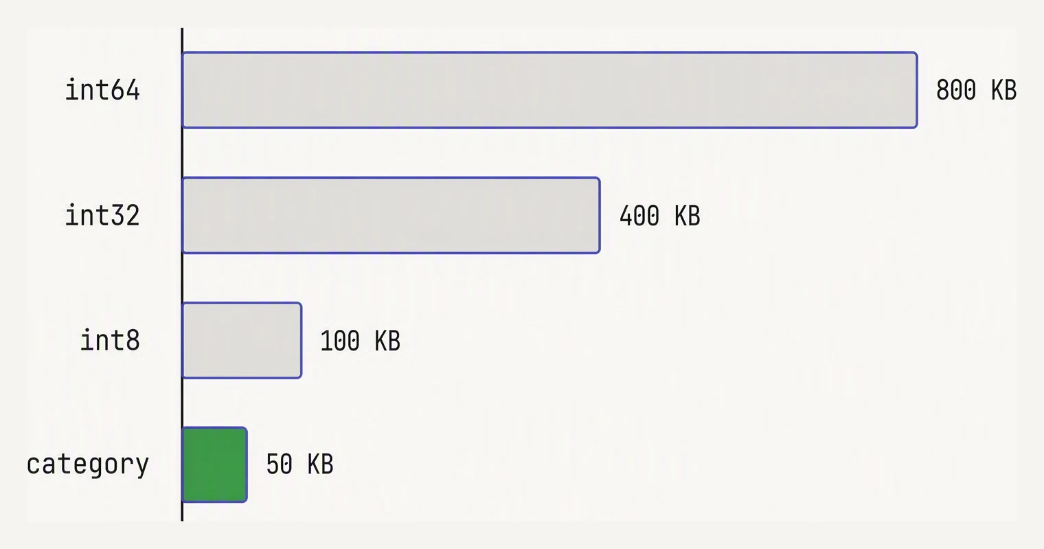
Same data, four dtypes. The column doesn’t change — the bill does.
You can’t shrink what you can’t see, and pandas has two views of memory that disagree. df.info()
gives a quick estimate. df.info(memory_usage='deep') walks into the object columns and counts the
actual bytes — which is the number you care about, because object columns are usually the elephant in
the room.
import pandas as pd
import numpy as np

rng = np.random.default_rng(42)
n = 100_000

# Synthetic log of API calls — the kind of thing you actually load at work
logs = pd.DataFrame({
    "request_id":  np.arange(n, dtype=np.int64),
    "status_code": rng.choice([200, 301, 400, 404, 500], size=n),
    "latency_ms":  rng.exponential(120.0, size=n),
    "region":      rng.choice(["us-east-1","us-west-2","eu-west-1","ap-south-1"], size=n),
    "method":      rng.choice(["GET","POST","PUT","DELETE"], size=n),
    "endpoint":    rng.choice(["/v1/users","/v1/orders","/v1/items","/v1/search"], size=n),
})

print("--- shallow (default) ---")
logs.info()
print()
print("--- deep ---")
logs.info(memory_usage="deep")
--- shallow (default) ---
<class 'pandas.core.frame.DataFrame'>
RangeIndex: 100000 entries, 0 to 99999
Data columns (total 6 columns):
# Column Non-Null Count Dtype
--- ------ -------------- -----
0 request_id 100000 non-null int64
1 status_code 100000 non-null int64
2 latency_ms 100000 non-null float64
3 region 100000 non-null object
4 method 100000 non-null object
5 endpoint 100000 non-null object
dtypes: float64(1), int64(2), object(3)
memory usage: 4.6+ MB
--- deep ---
<class 'pandas.core.frame.DataFrame'>
RangeIndex: 100000 entries, 0 to 99999
Data columns (total 6 columns):
# Column Non-Null Count Dtype
--- ------ -------------- -----
0 request_id 100000 non-null int64
1 status_code 100000 non-null int64
2 latency_ms 100000 non-null float64
3 region 100000 non-null object
4 method 100000 non-null object
5 endpoint 100000 non-null object
dtypes: float64(1), int64(2), object(3)
memory usage: 20.8 MBLook at the two memory lines: 4.6+ MB versus 20.8 MB. That little + in the shallow estimate is
pandas admitting it didn’t look inside the object columns — it counted only the pointers, not the
strings those pointers reach. The deep number, 20.8 MB, is the truth, and it’s more than four times
larger.
On real logs and tabular dumps, the object columns routinely dwarf everything else combined.
Downcast numerics
Start with the easy win. int64 can count up to ±9.2 quintillion; an HTTP status code needs nine
bits. Pandas reads in the safe-and-large dtype because at read time it doesn’t know your ranges — but
you do, so you pick the right-sized type afterward.
import pandas as pd
import numpy as np

rng = np.random.default_rng(42)
n = 100_000

logs = pd.DataFrame({
    "request_id":  np.arange(n, dtype=np.int64),
    "status_code": rng.choice([200, 301, 400, 404, 500], size=n).astype(np.int64),
    "latency_ms":  rng.exponential(120.0, size=n).astype(np.float64),
})

def mem_mb(df):
    return df.memory_usage(deep=True).sum() / 1024 / 1024

print(f"before: {mem_mb(logs):.2f} MB")
print(logs.dtypes)

# status_code fits in a small unsigned int
logs["status_code"] = pd.to_numeric(logs["status_code"], downcast="unsigned")
# latency_ms doesn't need float64 precision for analytics
logs["latency_ms"]  = pd.to_numeric(logs["latency_ms"], downcast="float")
# request_id is monotonic 0..n — uint32 reaches 4.3 billion
logs["request_id"]  = pd.to_numeric(logs["request_id"], downcast="unsigned")

print()
print(f"after:  {mem_mb(logs):.2f} MB")
print(logs.dtypes)
before: 2.29 MB
request_id int64
status_code int64
latency_ms float64
dtype: object
after: 0.95 MB
request_id uint32
status_code uint16
latency_ms float32
dtype: objectFrom 2.29 MB to 0.95 MB — better than half, and not a single value changed.
pd.to_numeric(..., downcast=...) inspects the actual range of the column and chooses the smallest
dtype that still fits it. Pass "integer", "unsigned", or "float" depending on what the column
holds.
Quick reference
| Dtype | Range | Bytes per value |
|---|---|---|
| int8 / uint8 | -128..127 / 0..255 | 1 |
| int16 / uint16 | ±32k / 0..65k | 2 |
| int32 / uint32 | ±2.1B / 0..4.3B | 4 |
| int64 (default) | ±9.2 quintillion | 8 |
| float32 | ~7 decimal digits | 4 |
| float64 (default) | ~15 decimal digits | 8 |
For analytics, float32 is almost always enough. The only times you genuinely need float64 are
scientific computing, financial math where the last cent matters, or long chains of multiplications
where rounding error compounds.
Categorical — the biggest win for repeated strings
Downcasting numbers is the warm-up. The real prize is strings. If a column has 100,000 rows but only four distinct values, it has no business being stored as 100,000 separate Python strings. Examples include:
regionmethodstatuscountrysegment
The categorical dtype stores each unique value once in a small lookup table and represents every
row as a tiny integer index into that table. A hundred thousand copies of "us-east-1" collapse into
a hundred thousand one-byte codes plus a handful of stored strings.
import pandas as pd
import numpy as np

rng = np.random.default_rng(42)
n = 100_000

logs = pd.DataFrame({
    "region":   rng.choice(["us-east-1","us-west-2","eu-west-1","ap-south-1"], size=n),
    "method":   rng.choice(["GET","POST","PUT","DELETE"], size=n),
    "endpoint": rng.choice(["/v1/users","/v1/orders","/v1/items","/v1/search"], size=n),
})

def mem_mb(df):
    return df.memory_usage(deep=True).sum() / 1024 / 1024

print(f"object dtype:      {mem_mb(logs):.2f} MB")

for col in ["region", "method", "endpoint"]:
    logs[col] = logs[col].astype("category")

print(f"categorical dtype: {mem_mb(logs):.2f} MB")
print()
print(logs.dtypes)
print()
print("region categories:", logs["region"].cat.categories.tolist())
object dtype: 18.48 MB
categorical dtype: 0.29 MB
region category
method category
endpoint category
dtype: object
region categories: ['ap-south-1', 'eu-west-1', 'us-east-1', 'us-west-2']18.48 MB down to 0.29 MB — past 20x, all the way to roughly 64x smaller. That’s the answer
to the prediction. It’s so dramatic precisely because the cardinality is so low: four values spread
across 100,000 rows means 99,996 of those strings were redundant.
Notice too that the categories come back sorted (ap-south-1, eu-west-1, …) — pandas keeps them
in a defined order, which is exactly what you want when a category is genuinely ordinal, like
["low","medium","high"].
And the saving isn’t only space. Categoricals also speed up groupby, merge, and value_counts on
those columns, because pandas gets to compare small integers instead of whole strings.
When NOT to use categorical
- The column is high cardinality — most values unique, like user IDs, UUIDs, or free-text comments. The lookup table grows as large as the data, so categorical adds overhead for no benefit.
- You’ll be string-manipulating the column heavily. Most
.stroperations have to materialize back to object dtype anyway, so you pay the conversion twice.
A rule of thumb: if df[col].nunique() / len(df) is below ~0.5, try categorical. Below 0.05 it is
almost always a win.
Loading huge files without breaking the loader
Everything so far shrinks a frame that’s already in memory. But sometimes the file is bigger than
RAM to begin with, or you need only a slice of it. read_csv has three knobs for exactly this.
usecols — load only the columns you need
df = pd.read_csv("huge.csv", usecols=["timestamp","user_id","amount"])If a 30-column file has 27 columns you’ll never touch, this is the single biggest speedup available — you skip parsing them entirely.
dtype — set dtypes at load time, skip the inference
df = pd.read_csv("logs.csv", dtype={
    "status_code": "uint16",
    "region":      "category",
    "method":      "category",
    "latency_ms":  "float32",
})
Now pandas never has to guess, and you skip the “load as object, then convert to category” round-trip — the round-trip that briefly doubles peak memory at exactly the moment you can least afford it.
chunksize — stream when the file won’t fit
For a file that simply cannot sit in RAM all at once, chunksize=N returns an iterator of
DataFrames. Each holds N rows. You process one, reduce it, discard it, and move on.
import pandas as pd
import numpy as np
import io

# Simulate a large CSV in memory
rng = np.random.default_rng(0)
n = 50_000
big_csv = io.StringIO()
pd.DataFrame({
    "user_id":  rng.integers(1, 1000, n),
    "amount":   rng.exponential(50, n).round(2),
    "country":  rng.choice(["IN","US","DE","JP"], n),
}).to_csv(big_csv, index=False)
big_csv.seek(0)

# Stream — never hold more than 5,000 rows at once
chunks = pd.read_csv(big_csv, chunksize=5_000, dtype={"country": "category"})

# Reduce as we go: total amount per country
totals = pd.Series(dtype="float64")
for chunk in chunks:
    chunk_totals = chunk.groupby("country", observed=True)["amount"].sum()
    totals = totals.add(chunk_totals, fill_value=0)

print(totals.round(2))
country
DE 620221.03
IN 639075.32
JP 619727.21
US 636170.59
dtype: float64The pattern is always the same three beats:
- read a chunk
- compute its partial reduction
- fold that into a running aggregate
It works beautifully for sums, counts, and group statistics — anything associative, where combining partial answers gives the same result as computing over the whole.
Putting it all together
Here is a real “slow load” you might inherit, fixed in a single call:
# Before — 1.2 GB in memory, 90 seconds to load
df = pd.read_csv("events.csv")

# After — 180 MB in memory, 25 seconds to load
df = pd.read_csv("events.csv",
    usecols=["timestamp","user_id","event_type","duration_ms","region"],
    dtype={
        "user_id":     "uint32",
        "event_type":  "category",
        "duration_ms": "float32",
        "region":      "category",
    },
    parse_dates=["timestamp"],
)
Same data, same downstream code — and about a 7x memory cut, which is typical for log-shaped or event-shaped data. Three ideas did all the work:
- load fewer columns
- declare narrow dtypes up front
- let the categoricals collapse the repeated strings
In one breath
Pandas defaults to oversized dtypes — int64, float64, and full Python-object strings — so a
modest CSV can balloon in RAM. Measure the real footprint with df.info(memory_usage='deep'), which
counts inside object columns instead of just their pointers.
Then shrink:
pd.to_numeric(..., downcast=...)rightsizes numbers (often halving them).astype("category")collapses low-cardinality string columns by tens of times because each repeated value becomes a one-byte code
For files larger than RAM, read_csv carries the same ideas to load time:
usecolsto skip columnsdtypeto declare types up frontchunksizeto stream and reduce associatively
Practice
Quick check
df.info() undercount memory for object columns?chunksize the right tool?A question to carry forward
Notice the quiet habit running through this whole lesson: logs["status_code"] = pd.to_numeric(...),
logs[col] = logs[col].astype("category") — we kept assigning a transformed column straight back into
the frame. That worked because logs was unambiguously its own DataFrame.
But the moment your frame is actually a slice of another one — subset = df[df["amount"] > 100] —
that same assignment gets murky. Are you editing the subset, or the original it was carved from?
Pandas often can’t tell either, and warns you with the single most confusing message in the whole
library: the SettingWithCopyWarning.
The next lesson takes that warning apart — what a “view” versus a “copy” really is, and why the warning
fires even when your code seems fine. It also covers the one-line habit (.loc, and .copy() at the
right moment) that makes it disappear for good.
Practice this in an interview
All questionsCategorical dtype stores a column's unique values once in a lookup table and represents each row as a small integer code, replacing repeated Python string objects. This cuts memory by an order of magnitude for low-cardinality string columns and accelerates GroupBy, sorting, and equality comparisons because pandas operates on integer codes rather than string comparisons.
CategoricalDtype stores a column as integer codes plus a small lookup table of unique values, dramatically reducing memory for low-cardinality string columns. It also enforces a fixed set of valid values, enables natural ordering, and speeds up groupby and sort operations.
eval() and query() parse expression strings and delegate evaluation to numexpr, which uses multi-threaded SIMD operations and avoids allocating intermediate arrays — giving 2-10x speedups on large DataFrames. They are most beneficial on DataFrames larger than a few hundred thousand rows where intermediate array allocation dominates; for small frames, the expression parsing overhead makes them slower than standard indexing.
The biggest wins come from converting low-cardinality string columns to category dtype (often 10x smaller), downcasting int64 and float64 to the smallest type that fits the data range, and using sparse arrays or chunked reads for data that doesn't need to live fully in memory.
pandas is slow primarily because Python loops bypass NumPy's vectorized C kernels, object-dtype columns prevent SIMD optimizations, and keeping entire datasets in memory limits scalability. The fixes are vectorization, categorical encoding, eval/query for large frames, chunking for out-of-core data, and switching to Polars or DuckDB for compute-heavy pipelines.