Data-centric ML — tweak the data, not the model
The fastest way to improve a stuck model is almost never another hyperparameter sweep. It's fixing the 50 mislabeled rows that are dragging the slice you care about into the dirt.
Written and reviewed by Shreyash Prashu Last reviewed
What you'll learn
- Why "more hyperparameter tuning" hits a wall and data work doesn't
- How to find label noise programmatically (confident learning)
- Slice analysis — finding the segment that's killing your model
- The 50-sample re-label trick that fixes the underperforming class
Before you start
The last lesson ended on a quiet realization: every time the baseline pointed at a problem — the war-story churn model, the implausible leakage gap — the cure was never a fancier algorithm but a closer look at the data. We promised to take that idea seriously and give it its name. Here it is.
You’ve got a model. F1 is stuck at 0.72. You’ve tried RandomForest, XGBoost, two grid searches, and started thinking about a “deeper model.” None of it moves the number more than a tenth of a point.
This is the moment Andrew Ng’s “data-centric AI” pitch becomes actionable. Data-centric AI is the practice of holding the model architecture fixed and improving performance by improving the data — labels, slices, and collection quality — rather than the algorithm. You stop touching the model and start touching the data. Specifically, the rows where the model is wrong — because that’s almost always where the labels are also wrong.
Why this works
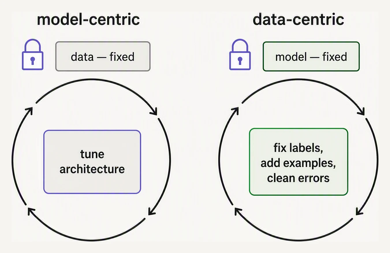
Same effort, two places to spend it. The data loop usually pays more.
ML libraries are very good. The gap between sklearn’s XGBoost defaults and a fully-tuned model is usually 1–3 F1 points. The gap between your labeled dataset and a correctly labeled dataset is often 5–15.
Most “messy real-world data” is messy in the labels, not just the features. Annotators are inconsistent, definitions drift over time, edge cases get inherited from a previous team and never re-litigated. Your model is dutifully learning the noise.
Tuning hyperparameters polishes the model on a noisy target. Fixing labels gives the model a cleaner target to learn. Guess which one moves the needle.
Step 1 — slice your eval set
Before you fix anything, find out which rows are killing you. Overall F1 of 0.72 doesn’t tell you whether you’re failing uniformly or whether one customer segment is at 0.4 and dragging the average down.
import numpy as np

from sklearn.datasets import make_classification
from sklearn.linear_model import LogisticRegression
from sklearn.model_selection import train_test_split
from sklearn.metrics import f1_score

X, y = make_classification(
    n_samples=3000, n_features=8, n_informative=4,
    weights=[0.7, 0.3], random_state=0,
)
# Pretend feature 0 encodes "customer segment" (3 buckets).
segments = np.digitize(X[:, 0], bins=[-0.5, 0.5])  # 0, 1, or 2

X_tr, X_te, y_tr, y_te, seg_tr, seg_te = train_test_split(
    X, y, segments, test_size=0.3, stratify=y, random_state=0,
)
model = LogisticRegression(max_iter=1000).fit(X_tr, y_tr)
pred = model.predict(X_te)

print(f"overall F1: {f1_score(y_te, pred):.3f}\n")
for s in (0, 1, 2):
    mask = seg_te == s
    if mask.sum() > 0:
        print(f"segment {s} (n={mask.sum():4d}): F1 = {f1_score(y_te[mask], pred[mask], zero_division=0):.3f}")
overall F1: 0.596
segment 0 (n= 369): F1 = 0.674
segment 1 (n= 213): F1 = 0.718
segment 2 (n= 318): F1 = 0.372Look at what the average hid. The headline F1 of 0.596 made the model look mediocre-everywhere — but it isn’t. Segments 0 and 1 are perfectly respectable at 0.674 and 0.718; the entire drag comes from segment 2, sitting at 0.372, less than half of segment 1. That is a completely different diagnosis than “the model is bad.” It is a targeted problem with a targeted fix: go get better labels for segment 2. You could never have seen this from the single 0.596 — the average is exactly the number that camouflages the segment killing you.
Step 2 — find label noise programmatically
You don’t have time to look at every row. You need the rows most likely to be mislabeled — i.e. the rows your model is confidently wrong about. If the model says “definitely class 1” with probability 0.97 but the label says class 0, one of two things is true: the model is wrong, or the label is wrong. Worth a human eyeballing.
This is the core idea behind confident learning — an algorithm that
finds likely mislabeled rows by looking for confident model disagreement
with the recorded label (implemented in the
cleanlab library). The
production version uses cross-validated out-of-fold probabilities to avoid
the model just memorising its own training set, but the spirit is the
same.
import numpy as np
import pandas as pd

from sklearn.datasets import make_classification
from sklearn.linear_model import LogisticRegression
from sklearn.model_selection import cross_val_predict

X, y = make_classification(n_samples=2000, n_features=6, random_state=0)
# Inject 5% label noise: flip the label on a random 5% of rows.
rng = np.random.default_rng(0)
noisy_idx = rng.choice(len(y), size=int(0.05 * len(y)), replace=False)
y_noisy = y.copy()
y_noisy[noisy_idx] = 1 - y_noisy[noisy_idx]

# Out-of-fold predicted probabilities — the model never sees a row's own label.
proba = cross_val_predict(
    LogisticRegression(max_iter=1000), X, y_noisy, cv=5, method="predict_proba",
)
confidence_in_label = proba[np.arange(len(y_noisy)), y_noisy]

# A row is 'suspicious' when the model is confident in a DIFFERENT class.
df = pd.DataFrame({
    "label": y_noisy,
    "predicted": proba.argmax(axis=1),
    "conf_in_label": confidence_in_label,
    "is_actually_corrupted": np.isin(np.arange(len(y_noisy)), noisy_idx),
})

suspects = df.sort_values("conf_in_label").head(10)   # 10 least-confident-in-label
print(suspects.to_string())
print(f"\n{suspects['is_actually_corrupted'].sum()} / 10 of these are real flips")
label predicted conf_in_label is_actually_corrupted
144 0 1 0.002001 True
1200 0 1 0.004165 True
1381 1 0 0.004819 True
671 0 1 0.006017 True
1669 0 1 0.006374 True
1068 0 1 0.007372 True
1342 1 0 0.008259 True
782 0 1 0.008336 True
1553 0 1 0.009411 True
1745 0 1 0.009657 True
10 / 10 of these are real flipsEvery single one of the ten most-suspicious rows is a genuine corrupted label — is_actually_corrupted is True
all the way down. Read the columns: row 144 is recorded as label 0, yet the model — which never saw row 144’s own
label, thanks to out-of-fold prediction — assigns it just 0.002 confidence in being a 0. The model is
screaming “this is the wrong class,” and it is right. Of course, perfect 10/10 is the very top of the list; push
deeper into the top ~200 suspects in a real project and the hit rate falls, but you would still typically find
20–40% genuine mistakes — and you would fix them.
Step 3 — re-label the slice that’s hurting
Now combine the two ideas. Find suspicious rows in the underperforming slice. Spend your annotation budget where it’ll move your metric.
# Pseudocode for what you'd do in a real project:
# 1) Compute slice-level F1.
# 2) Within the worst slice, sort by 'confidence in current label' ascending.
# 3) Take the bottom 50 — these are the rows your model thinks are mislabeled
#    in the slice you care most about.
# 4) Send those 50 to an annotator with the original input + your prediction.
# 5) Update labels, retrain, re-evaluate.
In practice you’ll find that 50 carefully chosen, carefully-relabeled rows move a slice-level F1 by 0.05–0.15, while another hyperparameter sweep moves the overall F1 by 0.005. The leverage is not even close.
A war story — recall on a niche class
A document-classification team had ~12 categories. Overall accuracy was 0.88. One class — “regulatory notice” — had recall of 0.41. The team spent two sprints on it: oversampling, class weights, focal loss, more data. Nothing got recall above 0.5.
A new engineer sliced the training set and pulled up the 30 most confidently-misclassified “regulatory notice” documents. About half of them weren’t actually regulatory notices — they were customer complaints about regulation. The label definition had drifted between two annotation batches. Once those 30 documents were corrected (and ~50 more identified via the same confident-learning approach), recall on that class jumped to 0.78 with no model change.
The fix was three days of annotation. The previous two sprints were trying to teach the model an inconsistent definition harder.
When to NOT do data work
Data-centric isn’t a dogma. Hyperparameter tuning and architecture choice still matter when:
- Your baselines are already strong and you’re squeezing the last 1–2%.
- You have very clean labels (medical imaging with senior radiologist consensus, say) and the model genuinely is the bottleneck.
- The labels are objectively defined by code (e.g. “did the user click” — there’s no ambiguity to clean).
In every other case — and especially anywhere humans are part of the labeling loop — fix the data first.
In one breath
When a model is stuck and more tuning won’t move it, go data-centric: slice the eval set to find where it fails (the 0.596 average hid segment 2 at 0.372), use confident learning to surface the rows the model is confidently disagreeing with their recorded label (the top 10 suspects were 10/10 genuine flips), re-label the worst rows in the worst slice, and you typically move a slice F1 by 0.05–0.15 — leverage a hyperparameter sweep cannot touch, because you are cleaning the target instead of polishing the model against noise.
Practice
Before the quiz, connect the two tools. The slice analysis found segment 2 (F1 0.372) as the underperformer, and confident learning found the most-likely-mislabeled rows. In your own words, why is running confident learning within segment 2 — rather than across the whole dataset — the move that spends a fixed annotation budget best? Then the war story: recall on “regulatory notice” was stuck at 0.41 through two sprints of oversampling and focal loss — what single thing had actually gone wrong, and why could no amount of model-tuning fix it?
Quick check
A question to carry forward
Notice the shape of every fix in this lesson. We found bad data after it had already trained a worse model, then
cleaned up after the fact — slice, suspect, re-label, retrain. That works, but it is firefighting: the corrupted
income-in-cents column, the drifted “regulatory notice” definition, the annotator inconsistency all got in
before anyone noticed.
So the question to carry forward is whether we can stop the bad data at the door instead of mopping up downstream. If most of what goes wrong is an upstream team silently renaming a column, flipping a unit, or starting to send nulls — could we write down, in advance, exactly what a dataset is allowed to look like, and make the pipeline reject anything that violates it before the model ever sees it? That enforceable, upstream agreement is a data contract, and it is the final lesson of this chapter.
Practice this in an interview
All questionsThe most common cause is training-serving skew: the distribution of features at serving time differs from the training data. The fix requires instrumenting the pipeline to log serving inputs, compare their distribution to training data, and identify whether the gap is due to data drift, feature engineering bugs, label leakage, or infrastructure inconsistencies.
Work top-down: start at the model layer with quantization, distillation, or routing cheaper models for easy requests, since model choices drive every downstream cost. Then optimize the runtime with batching, caching, and techniques like prompt caching for LLMs, and finally match infrastructure to the load using autoscaling on queue depth and spot or batch capacity. Track cost per token or per prediction alongside latency percentiles and accuracy so optimizations never silently degrade quality.
Freeze a representative test set before experimentation, then use only development data for preprocessing, feature selection, tuning, and model comparison. Fit every learned transformation inside each cross-validation fold, choose the model on development data, and evaluate the frozen choice on the test set once, using group or forward-chaining splits when rows are related or time-ordered.
Open-ended ML problems require scoping before modelling: translate the vague ask into a measurable business objective, identify which user interaction has the highest improvement potential, formulate it as a concrete ML task with a defined label and evaluation metric, then propose the simplest viable model first. Jumping to model architecture before this scoping is the most common interview failure mode.