Feature stores — when you need one, when you don't
The online/offline skew problem in one sentence, then a runnable Feast-shaped feature pipeline. Plus the honest answer to 'do we need a feature store?' (usually: no — until you do).
Written and reviewed by Shreyash Prashu Last reviewed
What you'll learn
- The training/serving skew problem — why a SQL query that worked offline silently breaks online
- Offline store vs online store — the two halves and why both exist
- Defining a feature view with a Feast-shaped API
-
get_historical_features(training) vsget_online_features(serving) — same definition, two reads - When a feature store is the right answer, and when it's premature infrastructure
Before you start
The last lesson left a model server running on a cluster and a question hanging over it: the request that arrives carries only a user id, but the model wants features — 30-day session counts, days-since-last-purchase. Those features must be computed in milliseconds and, crucially, computed exactly the way training computed them. Otherwise, the training-serving skew we met long ago silently wrecks it.
We asked where those request-time features come from and how you guarantee they match. This lesson is the system built to answer all of it at once.
A senior ML engineer once described the problem like this. The data scientist wrote a SQL query that joined three tables, computed a 30-day rolling average of user activity, and trained a churn model that hit 0.87 AUC. Six months later, the same model in production is getting 0.71 AUC, and nobody can figure out why.
It turns out the production feature service computes the same “30-day
rolling average” using a slightly different time window
(now() - INTERVAL 30 DAY instead of the training query’s
event_date BETWEEN snapshot_date - 30 AND snapshot_date). The
features look the same. They aren’t.
That’s training/serving skew. It’s the single most common failure mode in production ML, and it’s what feature stores were invented to fix.
The mental model
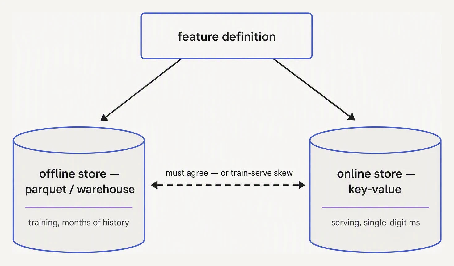
One definition, two stores — that is the whole point.
A feature store has two halves, and both halves answer the same question — “what was feature X for entity Y at time T?” — using very different infrastructure.
| Half | What it stores | Read latency | Used for | Typical backing |
|---|---|---|---|---|
| Offline store | Historical feature values, point-in-time | Minutes | Training, backfills | Parquet on S3, BigQuery, Snowflake, Delta |
| Online store | Latest feature values per entity | < 10 ms | Real-time inference | Redis, DynamoDB, Bigtable, RocksDB |
The whole point: one feature definition, two reads. You define
user_thirty_day_activity once. Training reads it from the offline
store with full history. Serving reads it from the online store at
inference time. The store guarantees they’re computed the same way.
Skew goes away because it can’t appear — by construction, both reads use the same upstream computation.
Drag the prediction time — see which value each store serves
Feature: user_7d_purchase_count. The offline store (top) is recomputed by a batch job every 4 hours — stale between runs. The online store (bottom) is updated by a streaming pipeline within seconds. Move the cursor to the moment a prediction fires; see the value each store returns. When they differ, you have training–serving skew.
At 6:30am, training reads 15 (last batch run) but serving reads 13 (current stream). The model was trained on data that looks systematically higher — online activity has cooled since the last batch run. That's the skew. A feature store removes it by enforcing one definition for both reads.
A feature view, Feast-shaped
Feast is the open-source default. The shape of its API has become the industry’s lingua franca even when teams use other stores.
# feature_repo/features.py — what your feature definitions actually look like
from datetime import timedelta
from feast import (
    Entity, FeatureView, Field, FileSource, ValueType, FeatureService,
)
from feast.types import Float32, Int64, String

# 1) Entities — the "thing" features are attached to.
user = Entity(name="user_id", value_type=ValueType.INT64, description="User primary key")

# 2) Source — where the offline data lives (here a Parquet file; in prod, BQ/Snowflake/S3).
user_activity_source = FileSource(
    path="s3://yourorg-features/user_activity.parquet",
    timestamp_field="event_timestamp",
    created_timestamp_column="created_ts",
)

# 3) Feature view — the unit of definition. Names, types, freshness, TTL.
user_activity_fv = FeatureView(
    name="user_activity_features",
    entities=[user],
    ttl=timedelta(days=2),     # online value is stale after 2 days of no update
    schema=[
        Field(name="thirty_day_session_count", dtype=Int64),
        Field(name="seven_day_avg_session_minutes", dtype=Float32),
        Field(name="days_since_last_purchase", dtype=Int64),
        Field(name="lifetime_purchases", dtype=Int64),
    ],
    source=user_activity_source,
    online=True,
)

# 4) Feature service — what your model actually consumes (a "view of views")
churn_risk_v1 = FeatureService(
    name="churn_risk_v1",
    features=[user_activity_fv],
)
That’s the entire contract. The same user_activity_fv definition
backs both training reads and online lookups.
Training — get_historical_features
For training, you have a list of (entity, label, timestamp) rows. You ask the store: “for each of these rows, give me the feature values as they were at that exact timestamp.”
This is point-in-time correctness — the killer feature. Without it, you accidentally use future information to predict the past, and your offline AUC ends up wildly higher than production performance.
# Training-time read — features as of each row's event_timestamp
from feast import FeatureStore
import pandas as pd

fs = FeatureStore(repo_path="feature_repo/")

# Your training spine: (user_id, label, when-the-prediction-was-made)
entity_df = pd.read_parquet("training_labels.parquet")
# columns: user_id, churned_within_30_days, event_timestamp

training_df = fs.get_historical_features(
    entity_df=entity_df,
    features=fs.get_feature_service("churn_risk_v1"),
).to_df()
# training_df now has the original columns + the feature columns,
# each feature value taken at-or-before its row's event_timestamp.
Two non-obvious wins:
- You can’t accidentally leak future state, because Feast enforces “no
feature value with
event_timestamp> the row’s timestamp.” - You can re-train on any historical date by changing
entity_df’s timestamps. Time-travel is built in.
Serving — get_online_features
For real-time inference, you have a single entity (a user_id) and
need the latest values, fast.
# Serving-time read — latest values, low latency
features = fs.get_online_features(
    features=fs.get_feature_service("churn_risk_v1"),
    entity_rows=[{"user_id": 4242}],
).to_dict()

# features = {
#   "user_id": [4242],
#   "thirty_day_session_count": [27],
#   "seven_day_avg_session_minutes": [13.4],
#   "days_since_last_purchase": [9],
#   "lifetime_purchases": [4],
# }

model_input = [
    features["thirty_day_session_count"][0],
    features["seven_day_avg_session_minutes"][0],
    features["days_since_last_purchase"][0],
    features["lifetime_purchases"][0],
]
score = model.predict_proba([model_input])[0][1]
A separate process — feast materialize — periodically computes and
pushes the latest feature values from the offline store into the online
store (hence “materialize”: turning a logical definition into stored,
ready-to-read values). That’s the only piece of infrastructure the
feature store is asking you to operate.
A runnable worked example
You can’t run the full Feast stack in the browser (it needs an online store and a materialize job), but you can run a faithful shape-of-it that demonstrates the duality. Same feature definition, two reads, both giving you the right answer.
# A Feast-shaped feature pipeline (the real thing needs: pip install feast).
# Same feature definition, two reads. Builds intuition for offline vs online.
from datetime import datetime, timedelta
from typing import List, Dict, Any
import pandas as pd
import numpy as np

# ----- 1) Fake source data (in prod this is a Parquet file on S3) -----
np.random.seed(0)
records = []
for user_id in range(1, 21):
    for day in range(60):
        records.append({
            "user_id": user_id,
            "event_timestamp": datetime(2026, 3, 1) + timedelta(days=day),
            "sessions_today": int(np.random.poisson(2)),
            "minutes_today": float(np.random.gamma(2, 5)),
        })
source = pd.DataFrame(records)
print("source rows:", len(source))

# ----- 2) The 'feature view': a transformation + entity + timestamp -----
def materialize(source: pd.DataFrame) -> pd.DataFrame:
    """Compute the rolling features per user, per day. Same function
    powers both reads."""
    out = source.sort_values(["user_id", "event_timestamp"]).copy()
    out["thirty_day_session_count"] = (
        out.groupby("user_id")["sessions_today"]
           .rolling(30, min_periods=1).sum().reset_index(level=0, drop=True).astype(int)
    )
    out["seven_day_avg_session_minutes"] = (
        out.groupby("user_id")["minutes_today"]
           .rolling(7, min_periods=1).mean().reset_index(level=0, drop=True)
    )
    return out[["user_id", "event_timestamp",
                "thirty_day_session_count", "seven_day_avg_session_minutes"]]

features_table = materialize(source)

# ----- 3) Offline read — point-in-time join (training) -----
def get_historical_features(entity_df: pd.DataFrame,
                            features: pd.DataFrame) -> pd.DataFrame:
    """For each (entity, ts) in entity_df, take the latest feature row
    where features.event_timestamp <= ts. This is the point-in-time
    correctness Feast gives you for free."""
    rows = []
    for _, row in entity_df.iterrows():
        candidates = features[
            (features["user_id"] == row["user_id"])
            & (features["event_timestamp"] <= row["event_timestamp"])
        ]
        if candidates.empty:
            rows.append({**row.to_dict(),
                         "thirty_day_session_count": None,
                         "seven_day_avg_session_minutes": None})
        else:
            latest = candidates.iloc[-1]
            rows.append({
                **row.to_dict(),
                "thirty_day_session_count": int(latest["thirty_day_session_count"]),
                "seven_day_avg_session_minutes": float(latest["seven_day_avg_session_minutes"]),
            })
    return pd.DataFrame(rows)

# A training spine — what features looked like on the day each label was created.
training_labels = pd.DataFrame([
    {"user_id": 3,  "event_timestamp": datetime(2026, 3, 20), "churned": 1},
    {"user_id": 7,  "event_timestamp": datetime(2026, 4, 5),  "churned": 0},
    {"user_id": 12, "event_timestamp": datetime(2026, 4, 15), "churned": 1},
])
training_df = get_historical_features(training_labels, features_table)
print("\n--- training-time read (point-in-time correct) ---")
print(training_df.to_string(index=False))

# ----- 4) Online read — latest value, fast lookup (serving) -----
# In real Feast: features live in Redis/DynamoDB keyed by entity.
online_store: Dict[int, Dict[str, Any]] = {}
for uid, group in features_table.groupby("user_id"):
    latest = group.iloc[-1]
    online_store[int(uid)] = {
        "thirty_day_session_count": int(latest["thirty_day_session_count"]),
        "seven_day_avg_session_minutes": float(latest["seven_day_avg_session_minutes"]),
        "event_timestamp": latest["event_timestamp"],
    }

def get_online_features(user_ids: List[int]) -> List[Dict[str, Any]]:
    """O(1) per entity. Real Feast does this in <10ms over Redis."""
    return [online_store.get(uid, {}) for uid in user_ids]

print("\n--- serving-time read (latest, low latency) ---")
for uid, vals in zip([3, 7, 12], get_online_features([3, 7, 12])):
    print(f"user {uid}: {vals}")

# ----- 5) The whole point: training and serving used the SAME materialize() -----
# If we change the transformation, both reads change together.
# Skew is impossible by construction.
print("\nfeature definition lives in materialize() — used by both reads.")
source rows: 1200
--- training-time read (point-in-time correct) ---
user_id event_timestamp churned thirty_day_session_count seven_day_avg_session_minutes
3 2026-03-20 1 37 13.522594
7 2026-04-05 0 65 13.937068
12 2026-04-15 1 57 13.069629
--- serving-time read (latest, low latency) ---
user 3: {'thirty_day_session_count': 54, 'seven_day_avg_session_minutes': 11.866392238503733, ...}
user 7: {'thirty_day_session_count': 60, 'seven_day_avg_session_minutes': 9.287582099317925, ...}
user 12: {'thirty_day_session_count': 57, 'seven_day_avg_session_minutes': 10.770575341781798, ...}
feature definition lives in materialize() — used by both reads.Look at user 3 in both reads, because the difference is the whole idea. The training read returns 37 sessions — the value as of the label date, 2026-03-20. The serving read returns 54 — the latest value, as of 2026-04-29.
Different numbers, and that’s correct: training must see the world as it was when the label was made (the point-in-time join refuses any feature stamped after the row’s timestamp, so no future leaks in). Serving wants the freshest value available right now.
The thing that cannot differ is how each number was computed — both reads ran the identical materialize().
Change that one function and both halves change together, which is precisely why skew becomes impossible rather than
merely unlikely. Real Feast doesn’t recompute on the fly; it materializes into the online store on a schedule. But
the contract — one definition, two reads — is exactly this.
When a feature store is the right answer
A feature store earns its weight when several of these are true:
- You have many models reusing the same features. The “definition once, reads everywhere” win compounds with reuse. With one model and four features, the wins are theoretical.
- You serve in real time (single-digit ms latency budgets). You need an online store.
- You’ve already shipped a model that drifted because training features and serving features diverged. You know the pain.
- Multiple teams contribute features and you need governance: ownership, lineage, freshness SLAs.
- You have point-in-time correctness needs — temporal features where using future data leaks.
When it’s premature infrastructure
Equally true:
- You have under five production models. The shared-definition payoff is small.
- You don’t serve in real time. If your inference is batch (nightly scoring), the offline store is your feature store — Parquet on S3 with snapshot dates does the job, and adding Feast on top is ceremony.
- Your features are simple aggregates from a single source. A view in Snowflake or BigQuery, materialized nightly, is cheaper to operate than a feature store.
- Nobody on the team will own the feature store. Like Kubeflow, Feast/Tecton needs an owner. An unmaintained feature store decays fast.
The managed vs. open-source landscape
| Option | What it is | Sweet spot |
|---|---|---|
| Feast | Open-source, BYO infra (Redis + S3 + your own materialize) | Teams with existing cloud infra; flexibility over hand-holding |
| Tecton | Managed feature platform with streaming, transformations, SLA monitoring | Real-time, multi-team, complex transformations |
| Databricks Feature Engineering | Feature store inside Databricks workspace | Already on Databricks; want one less integration |
| SageMaker Feature Store | AWS-native feature store with offline + online stores | Heavy SageMaker shops |
| Vertex AI Feature Store | GCP-native equivalent | Heavy Vertex shops |
| Just a warehouse view | Materialized SQL, no special framework | Batch scoring, fewer than 5 models, no real-time needs |
The pattern: the more of these you have, the more justification for a managed (Tecton, Databricks, SageMaker) option:
- models
- teams
- real-time needs
The more you’re a one-team shop with batch needs, the more “a table in Snowflake” is the right answer.
What never changes — the feature contract
Whatever you choose, the idea is the part you internalise:
- A feature is a named, typed, owned quantity attached to an entity at a timestamp.
- The definition of that feature is code — versioned, reviewed, tested.
- Training and serving read the same definition, never reimplement it.
You can do all three without Feast. You can fail at all three with Feast. The infrastructure is downstream of the discipline.
In one breath
A feature store exists to kill training-serving skew by enforcing one feature definition, two reads:
- an offline store (historical, point-in-time, minutes-latency — for training and backfills)
- an online store (latest value per entity, sub-10ms — for real-time inference)
Both are fed by the same computation so they can’t diverge. get_historical_features gives point-in-time-correct
training data (no future leaks), while get_online_features gives the freshest value fast, and a materialize job
pushes offline→online on a schedule.
But the discipline (a feature is versioned, owned code; training and serving never reimplement it) matters more than the tool. For one batch-scored model, a materialized warehouse view is your feature store.
Practice
Before the quiz, reconcile the two reads from the worked example. User 3 came back as 37 sessions from the training read but 54 from the serving read — and the lesson calls both correct. Explain why those should differ, and what would be alarming if they were instead computed by two different functions.
Then the judgment call the lesson hammers: you have one nightly-batch-scored model whose features come from a single Snowflake table — name the specific reason adopting Feast here is a liability, not an upgrade.
Quick check
get_historical_features?A question to carry forward
Take stock of the platform this chapter has assembled:
- Rented cloud machines
- a Kubernetes cluster
- Kubeflow pipelines
- a feature store with its online Redis layer and its scheduled materialize job
It is a genuinely powerful stack — and every single piece of it is running on hardware that bills you by the second, much of it on the most expensive silicon money can rent: GPUs.
So far we have talked about all of it as if it were free. It is emphatically not.
- A GPU fleet at 40% utilization burns more than half its cost on idle metal.
- A forgotten instance turns a weekend into a four-figure surprise.
- A model that costs more per prediction than it earns loses money faster the better it works.
So the question to carry forward, now that the platform exists, is the one the finance team is already asking:
- what does all this cost?
- where does the money actually leak?
- how does an ML engineer control it?
That is cost and FinOps for ML and GPUs, and it is the next lesson.
Practice this in an interview
All questionsA feature store is a shared data platform that computes, stores, and serves ML features consistently for both training and serving. It eliminates training-serving skew by ensuring the same transformation code runs in both contexts, and it reduces duplicated work by letting teams share and discover features across models.
DVC (and lakeFS) version raw datasets and model artifacts as immutable snapshots tied to Git commits, giving reproducibility and rollback. A feature store manages computed features for training and serving, its main job being to keep offline and online feature definitions in sync to prevent training-serving skew. They are complementary: DVC answers what data made this model, while a feature store answers how do I serve the same features consistently.
Training-serving skew is any mismatch between how features are computed during training and how they are computed at serving time, which silently degrades a model that looked fine offline. It arises when offline and online feature logic are implemented separately, for example a rolling average computed over a different window in each path. A feature store prevents it by keeping a single feature definition used for both batch training and online serving, so the same values and logic apply in both, and it supports point-in-time-correct retrieval to avoid leakage.
Feature engineering is creating, transforming, or selecting input variables so a model can capture patterns more easily. Common techniques include scaling, encoding categoricals, binning, interaction and ratio features, date/time decomposition, and domain-derived aggregates. It often matters more than the choice of algorithm because models can only learn from the signal present in their inputs.