Baselines — the first thing you build
Before you train a model, train the dumbest possible model. It's a floor, a leakage detector, and the thing that most often saves you from shipping a worse system.
Written and reviewed by Shreyash Prashu Last reviewed
What you'll learn
- The three baselines every project should start with
- How a baseline catches data leakage (and why that matters more than the floor)
- The "predict no-churn" story — when a baseline beats your tuned model
- How to wire baselines into your eval pipeline so they stay honest
Before you start
The last lesson left us with a deflating question: before you may call a model “good,” what exactly does it have to beat?
We hinted at the answer — not a rival model, but something far dumber and far more revealing. This lesson is that something.
A baseline is the simplest possible predictor you can build before
touching a real model — random guess, majority class, the mean of y,
or a hand-coded rule. It sets the floor: any model worth shipping must
beat it.
- If you can’t beat the baseline, you don’t have a model — you have an expensive way to underperform a constant.
- If you do beat it but only by 0.5%, you might have a model but you don’t have a business case.
- And if your model beats the baseline by forty points on a hard problem, that’s not a celebration — that’s almost always leakage.
Baselines do three jobs at once. Build them first, before anything else.
The three baselines you should always have
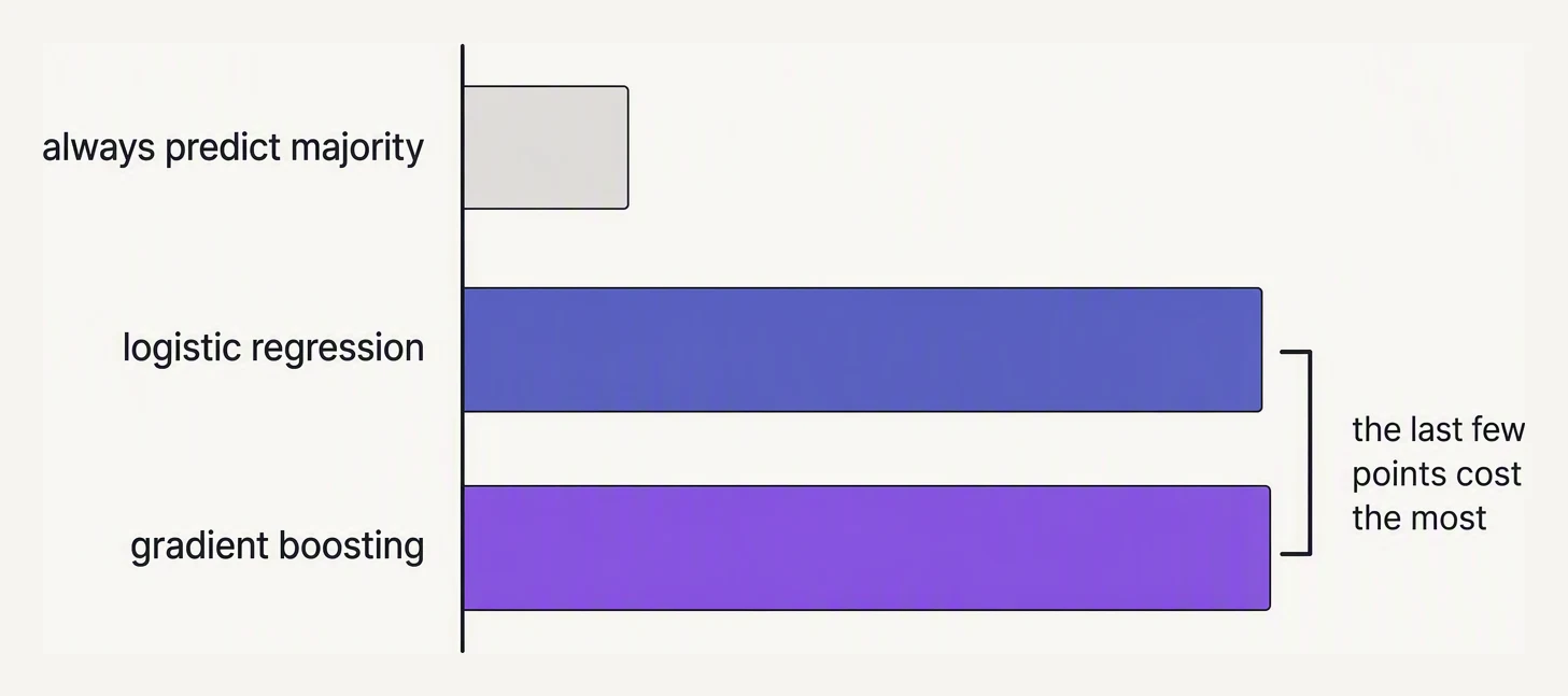
If you cannot beat the dumb answer, the complex one is not the problem.
You don’t pick one. You build all three and put them next to your model.
| Baseline | What it predicts | What it catches |
|---|---|---|
| Random | Uniform random label | Whether your model has any signal at all |
| Majority / mean | Always the most common class, or mean(y) for regression | The “constant predictor” floor that accuracy hides |
| Heuristic | A hand-coded rule (if revenue > X and last_login > 30d → churn) | Whether your model beats what a product manager could write |
The heuristic is the most important one. It’s the one that says “is this ML project worth shipping?”
Build them in 20 lines
import numpy as np

from sklearn.datasets import make_classification
from sklearn.dummy import DummyClassifier
from sklearn.linear_model import LogisticRegression
from sklearn.model_selection import train_test_split
from sklearn.metrics import accuracy_score, f1_score

# Simulate a churn dataset: 90% non-churners, 10% churners.
X, y = make_classification(
    n_samples=3000, n_features=10, n_informative=4,
    weights=[0.9, 0.1], random_state=0,
)
X_tr, X_te, y_tr, y_te = train_test_split(X, y, test_size=0.3, stratify=y, random_state=0)

rand = DummyClassifier(strategy="stratified", random_state=0).fit(X_tr, y_tr)  # random guess
maj  = DummyClassifier(strategy="most_frequent").fit(X_tr, y_tr)              # always majority
def heuristic(X):
    return (X[:, 0] < -0.5).astype(int)   # a hand-rolled rule on one feature

model = LogisticRegression(max_iter=1000).fit(X_tr, y_tr)   # the "real" model

for name, pred in [
    ("random       ", rand.predict(X_te)),
    ("majority     ", maj.predict(X_te)),
    ("heuristic    ", heuristic(X_te)),
    ("logistic_reg ", model.predict(X_te)),
]:
    print(f"{name}  acc={accuracy_score(y_te, pred):.3f}  f1={f1_score(y_te, pred, zero_division=0):.3f}")
random acc=0.806 f1=0.112
majority acc=0.897 f1=0.000
heuristic acc=0.678 f1=0.162
logistic_reg acc=0.913 f1=0.328Read that table slowly, because the whole lesson lives in it.
The majority baseline scores 0.897 accuracy just by predicting “not churned” for everyone — and its F1 is exactly 0.000, because it never catches a single churner.
Now look at the real model: 0.913 accuracy. On the accuracy column it has lifted things by a measly 1.6 points over a constant — if accuracy were your headline metric, you would be tempted to declare the project a wash.
But the F1 column tells the true story: the model goes from the majority’s 0.000 to 0.328, which means it is genuinely catching churners the constant could not.
Same two models, two completely different verdicts — and the only thing that revealed the difference was having the baselines sitting right next to the model.
This is the single most common failure mode in early-career ML work, and the baseline column is the only thing that surfaces it.
The floor — what “beating the baseline” actually means
A model is only worth shipping if it beats the baseline on the metric that matters — and which metric you pick can flip the verdict.
Look back at the table. On accuracy, the logistic model’s 0.913 sits barely above the majority’s 0.897; a skeptic could wave away those 1.6 points as noise and ask what the modelling actually bought.
On F1, the very same model jumps from a flat 0.000 to 0.328 — not a marginal nudge but the difference between catching no churners and catching a real share of them. Identical model, opposite stories.
The point isn’t the number. The point is that the baseline forces you to declare, out loud, which metric you are standing on — and then gives you a calibrated floor on exactly that one.
The leakage detector — the more important job
Imagine you trained a churn model and it hit 0.99 F1. Champagne, right?
No — find the bug.
Real churn problems on real data hit 0.6–0.8 F1. Anything dramatically higher means one of:
- A feature derived from the label snuck into the input (e.g., a
last_payment_attempted_atcolumn that only gets populated after churn). - Your train/test split leaked (the same user appears in both sets).
- Your test set is too small or unrepresentative.
- Time travel — a feature uses data from after the prediction time.
Baselines give you a sniff test. If random gets 0.05 and your model gets 0.99, the gap is implausible. Something in your data pipeline is letting the model peek at the answer. The baseline didn’t catch leakage directly, but it told you the gap was too big to be real.
The “predict no-churn” story
Here’s a war story that plays out somewhere every quarter.
A team is told to build a churn model. The label distribution is 95/5 (95% retain, 5% churn). They train an XGBoost. The notebook says “model accuracy: 94.2%.” They’re proud. They ship it to a Slack channel for review.
Senior engineer adds: “What does class_weight='balanced' and
DummyClassifier(strategy='most_frequent') give us?”
Twenty minutes later, the team comes back: the dummy model gets 95.0% accuracy. The XGBoost is worse than a constant. The team had spent two weeks tuning a model that was, on the metric they reported, underperforming “predict no for everyone.”
What actually went wrong: the XGBoost was occasionally predicting churn, and those predictions were mostly wrong because they hadn’t tuned the threshold or weighted the loss. The model was generating false positives without catching enough true positives to compensate.
Two things would have caught this on day one:
- Reporting the dummy baseline alongside the model.
- Reporting precision/recall, not accuracy, on an imbalanced problem.
The fix isn’t a better model. The fix is having the baseline in the eval report from the start.
Bake them into the pipeline
Don’t compute baselines once in a notebook and then forget about them. Every time you re-evaluate a model — every CI run, every retrain — the baselines run alongside, on the same eval set, and get reported in the same table.
A minimal pattern:
from sklearn.dummy import DummyClassifier
from sklearn.metrics import f1_score

def eval_with_baselines(X_tr, y_tr, X_te, y_te, model, heuristic_fn=None):
    results = {}
    for strat in ["stratified", "most_frequent"]:
        d = DummyClassifier(strategy=strat, random_state=0).fit(X_tr, y_tr)
        results[f"baseline_{strat}"] = f1_score(y_te, d.predict(X_te), zero_division=0)
    if heuristic_fn is not None:
        results["baseline_heuristic"] = f1_score(y_te, heuristic_fn(X_te), zero_division=0)
    results["model"] = f1_score(y_te, model.predict(X_te), zero_division=0)
    return results

# Smoke test on toy data
from sklearn.datasets import make_classification
from sklearn.linear_model import LogisticRegression
from sklearn.model_selection import train_test_split

X, y = make_classification(n_samples=2000, weights=[0.9, 0.1], random_state=0)
X_tr, X_te, y_tr, y_te = train_test_split(X, y, stratify=y, random_state=0)
model = LogisticRegression(max_iter=1000).fit(X_tr, y_tr)

print(eval_with_baselines(X_tr, y_tr, X_te, y_te, model,
                          heuristic_fn=lambda X: (X[:, 0] < -0.5).astype(int)))
{'baseline_stratified': 0.1415929203539823, 'baseline_most_frequent': 0.0, 'baseline_heuristic': 0.026845637583892617, 'model': 0.96}Every baseline lands near the floor:
- the stratified guess at 0.14,
- the majority at a flat 0.0,
- the hand-rolled heuristic at 0.03.
The model clears all three at 0.96.
This is clean synthetic data, so the gap is flattering; on a real churn problem you would expect something far more modest, and a 0.96 should make you suspicious, not proud — more on that below.
The shape is what matters: a single function that always returns the model’s score and the floor it had to clear, every single time it runs.
The output should always have a “model” entry that beats every baseline. If it doesn’t, the right CI behavior is to block the deploy. We’ll wire that into GitHub Actions later in this section.
In one breath
A baseline is the dumbest predictor you can write — random, majority/mean, or a hand-coded heuristic — and you build all three first because they do three jobs at once:
- they set a floor on the metric that actually matters (exposing the constant-predictor trap that accuracy hides),
- they act as a leakage detector (a model that beats a 0.05 baseline by jumping to 0.99 is almost certainly peeking at the answer),
- and baked into the eval pipeline they keep every future retrain honest.
Practice
Before the quiz, sit with the “predict no-churn” war story. A team shipped an XGBoost at 94.2% accuracy on a 95/5
split, and the most_frequent dummy quietly scored 95.0% — the tuned model was worse than a constant.
In your own words: which one number, reported on day one, would have stopped two weeks of wasted work? And the sharper one: in the smoke test above, the model hit F1 0.96 against near-zero baselines — why should that gap make you reach for the data pipeline rather than the champagne?
Quick check
A question to carry forward
So baselines hand you a floor — but notice how the war story actually got fixed, and how leakage actually gets fixed. In both cases the cure was never a fancier algorithm.
It was looking harder at the data: the label balance, the leaking feature, the contaminated split. The baseline kept pointing back at the data, not the model.
That points at the question to carry forward.
If the most reliable way to raise the floor is almost never a better model but a better dataset — cleaner labels, fixed slices, honest splits — then maybe we have been holding the whole craft backwards, tuning architectures when we should be tuning data.
The next lesson takes that idea seriously and names it: data-centric AI, the discipline of improving the model by improving everything except the model.
Practice this in an interview
All questionsWhen true labels are unavailable or arrive weeks late, you monitor leading indicators instead: input distribution drift, output score distribution shift, proxy business metrics, and inter-model disagreement. These act as early-warning signals before any labelled evaluation becomes possible.
Offline metrics often don't predict business impact, so you run a controlled online experiment: split live traffic between the current champion and the new challenger and compare a pre-registered business metric with a statistical significance test. You size the test for adequate power, watch guardrail metrics like latency and errors, and only ship if the lift is statistically and practically significant. Variance-reduction techniques like CUPED let you reach significance faster.
Work top-down: start at the model layer with quantization, distillation, or routing cheaper models for easy requests, since model choices drive every downstream cost. Then optimize the runtime with batching, caching, and techniques like prompt caching for LLMs, and finally match infrastructure to the load using autoscaling on queue depth and spot or batch capacity. Track cost per token or per prediction alongside latency percentiles and accuracy so optimizations never silently degrade quality.
Full retraining trains a fresh model from scratch on the latest data window, giving the cleanest result but at the highest cost and slowest cadence. Incremental or warm-start training continues from existing weights on new data, which is cheaper and faster but can accumulate drift and forgetting. Continual online learning updates the model continuously from a live stream for maximum freshness, at the cost of stability, harder evaluation, and vulnerability to bad or poisoned data.