Cost & FinOps for ML/GPU
GPU spend can become a board-level concern, and MLOps shares responsibility for making it visible and controllable. Learn how allocated capacity, utilization, workload shape, and unit economics determine the real cost of training and inference.
What you'll learn
- Why allocated GPU time, rather than useful compute, often drives GPU spend
- How to calculate cost per training run and cost per 1,000 inferences
- Which utilization, pricing, sizing, and autoscaling levers actually reduce cost
- How to recognize cost failures before they become a five-figure cloud bill
Before you start
It is Monday morning. The fraud model is no more accurate than it was on Friday, but the cloud bill is $3,840 higher. Someone left eight GPUs attached to a development endpoint. The endpoint received 19 requests all weekend.
Nothing crashed. No alert fired. The meter simply kept running.
That is the awkward truth about ML infrastructure: the expensive part often is not a spectacular training run. It is capacity that exists for a job that is waiting on data, a serving replica that is waiting on traffic, or a powerful GPU doing work a smaller one could do.
FinOps is the discipline of connecting cloud spending to engineering decisions. In ML, FinOps answers questions such as:
- Did this retraining run earn its $84 price?
- How much does one thousand predictions cost?
- Are we paying for a GPU because the model needs it, or because nobody changed the default?
- Can an interruption stop this job safely?
- Is the cheaper GPU actually cheaper once its slower runtime is included?
The goal is not to make every job as cheap as possible. The goal is to spend deliberately while meeting accuracy, latency, reliability, and compliance requirements.
The meter runs whether you use it or not
A cloud GPU is normally billed for the time the resource is allocated. The bill does not inspect whether your model was producing useful predictions during that time.
This explains GPU cost, not total ML infrastructure cost. CPU, memory, storage, networking, managed services, software licenses, and data transfer can also be substantial.
Utilization is not a standardized measure of useful capacity. A GPU-busy percentage often measures the fraction of sampled time with kernels active, not useful throughput. A value of 40% therefore cannot generally be interpreted as 60% of billable capacity being wasted.
Suppose a team allocates eight GPUs for 24 hours. For an internal comparison, assign a rate of $4 per GPU-hour:
allocated = 8 * 24 * 4
idle_equivalent = allocated * (1 - 0.40)

print(f"allocated: ${allocated:,.2f}")
print(f"idle-equivalent: ${idle_equivalent:,.2f}")
The output is:
allocated: $768.00
idle-equivalent: $460.80
That second number is an idle-equivalent estimate for screening. It is not a provider invoice line or proof that the remaining 60% was useless. A memory-bound workload can show low arithmetic utilization while still making progress; a data pipeline can leave the GPU waiting even though the overall job is healthy.
Use the estimate alongside throughput, queue time, and latency. A 40% metric paired with healthy throughput may describe an adequate system. A 70% metric paired with growing queues may describe one running hot but serving users badly.
The practical conclusion survives those caveats:
Before negotiating a lower GPU rate, find out why the GPUs are waiting.
Common causes include slow input pipelines, unbatched serving, a job occupying a whole GPU while using little memory, minimum replicas left running overnight, and distributed jobs waiting for their slowest worker. Pair utilization with throughput, queue depth, memory use, batch latency, and completion time.
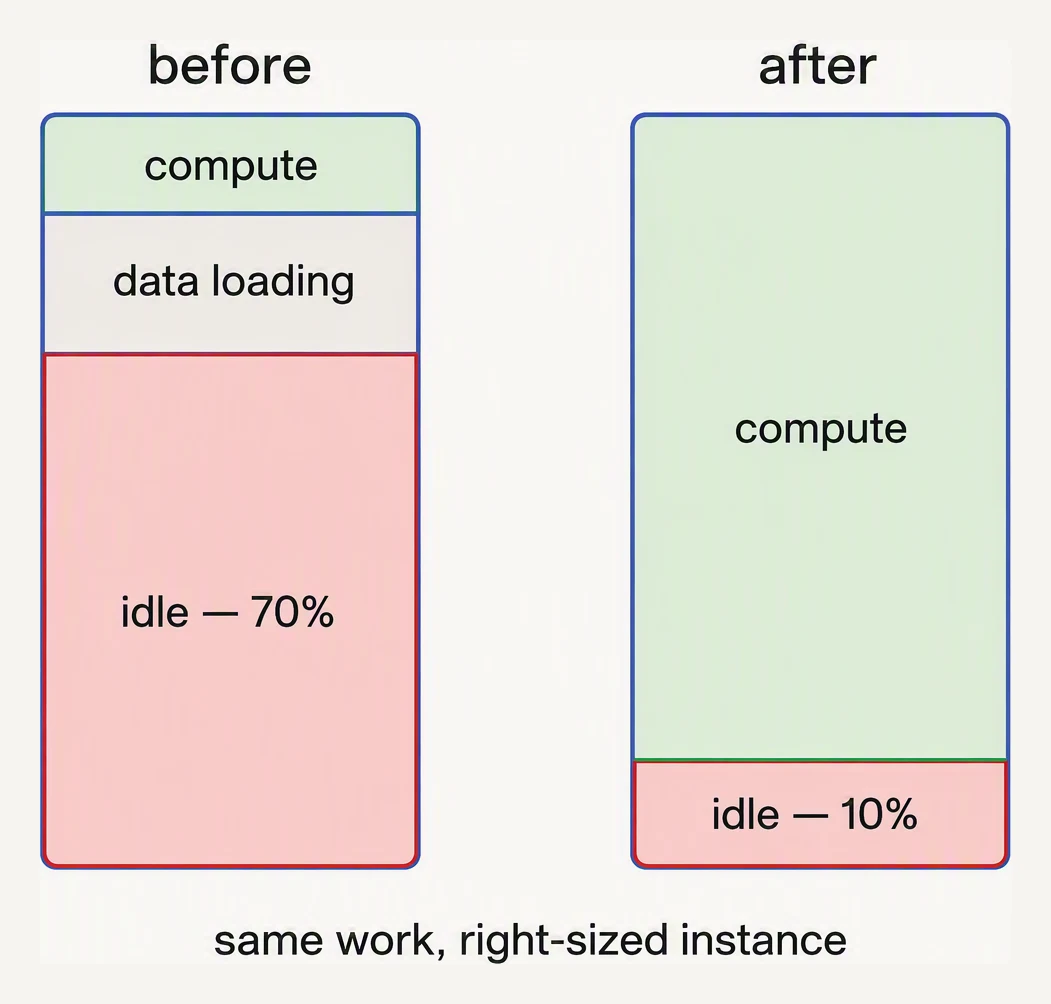
Illustrative: in an underutilized fleet, idle allocation can dominate GPU cost.
The calculator below is useful for a first estimate. Use your actual allocation, hourly rate, and utilization.
The meter runs whether you use it or not
Size a GPU fleet and watch the monthly burn — and how much of it is idle waste. GPU spend is the fastest-growing line on enterprise cloud bills, and utilization is where most of it leaks.
Cost is a workload calculation, not just a price calculation
The cheapest GPU-hour is not necessarily the cheapest completed job.
- GPU A costs $4 per hour and completes a run in 10 hours: $40.
- GPU B costs $7 per hour and completes it in 4 hours: $28.
A higher hourly price wins because the job finishes sooner. Measure cost per completed outcome, not only price per hour. The comparison changes if GPU B waits for data or the job is too small to benefit from its extra capacity.
For a training run, a useful first formula is:
run cost = accelerator-hours × accelerator rate + CPU-hours × CPU rate + memory-GB-hours × memory rate + storage cost + transfer cost + orchestration cost
Include setup overhead, retries, and failed attempts. A nightly retraining job might look like this:
- Four GPUs for six hours at $3.50 per GPU-hour: $84.
- CPU, memory, and orchestration overhead: $11.
- Storage and data transfer: $5.
- One failed run that consumed $18 before being retried.
The nightly cost is $118, not $84. If this happens 30 times, the monthly training bill is $3,540. The internal rate should include the costs your team is responsible for. For shared clusters, choose an allocation method—such as GPU-hours, reserved capacity, or measured usage—and document it. An honest estimate is better than false precision.
For serving, use cost per 1,000 homogeneous predictions for fixed-shape tasks. Requests should have broadly comparable input and output size, batching behavior, cache-hit rate, and retry rate. For generative models, report cost per input token and output token, or cost per representative request mix.
cost per 1,000 inferences = total serving cost / number of inferences × 1,000
Define the denominator: say whether it includes successful requests, retries, errors, cached responses, and items processed inside a batch. Measure the numerator and denominator over the same window.
Suppose a service runs two GPUs for a 30-day month, using 720 hours, at an internal rate of $3 per GPU-hour:
- GPU cost:
2 × 720 × $3 = $4,320. - Traffic: 1,000,000 predictions.
- GPU cost per 1,000 predictions:
$4,320 / 1,000,000 × 1,000 = $4.32.
Add CPU, memory, storage, and egress before calling that the real unit cost. If the business earns $5 per 1,000 predictions, the gross contribution before other costs is $0.68. If it earns $3, the service loses $1.32, even with excellent accuracy.
For internal models, use the business unit that matters: cost per document, approved application, or thousand support tickets.
Average cost spreads fixed capacity across all predictions. Marginal cost is the extra cost of one more prediction. Average cost shows whether the service is sustainable; marginal cost helps an autoscaler or product team decide what happens at the next traffic level. Report both where they differ.
The cost levers
Raise useful utilization
This is often the highest-leverage lever because it increases the work produced by capacity you already pay for.
For training, pack independent jobs onto available capacity with a scheduler. GPU sharing, time-slicing, or partitioning such as MIG can fit smaller workloads onto one accelerator when supported.
For inference, dynamic batching combines requests into one accelerator operation. It often improves efficiency, but requests wait briefly for a batch, increasing latency. Autoscaling can reduce replicas as traffic falls. Scale to zero removes serving capacity when there is no work, but cold starts, model loading, storage, and buffering still cost time and money. It fits development, scheduled jobs, and infrequently called endpoints better than a customer-facing service with a strict first-response target.
The target is the smallest reliable capacity that meets the service-level objective, not zero at any price.
Use spot or preemptible capacity where interruption is safe
Spot or preemptible instances are discounted spare capacity that the provider can reclaim. Discounts vary by provider, region, accelerator, and demand.
They suit checkpointed training, hyperparameter sweeps, batch feature generation, and offline evaluation. They are a poor default for latency-critical serving.
Checkpointing makes interruption survivable. Store model weights, optimizer and scheduler state, relevant random state, and data position in durable storage. A checkpoint every 15 minutes limits ordinary lost work to roughly 15 minutes; a checkpoint only at the end of a 12-hour run does not.
Commit only the baseline you can defend
Reserved or committed-use discounts make sense for predictable, sustained demand. Commit the normal floor and leave bursts flexible. If normal demand is two GPUs and the peak is eight, reserving eight means paying for six GPUs most of the year.
Calculate break-even utilization and include cancellation, regional, instance-family, and portability constraints. A discount on capacity nobody needs is still waste.
Right-size the accelerator
Match the accelerator to memory requirements, throughput, and parallelism. Test candidates using requests per second, p95 or p99 latency, batch size, peak memory, warm-up time, and cost per completed prediction.
Benchmark the complete serving topology. A smaller GPU that needs six replicas can cost more than one larger GPU, and a GPU at 85% utilization may lack the headroom needed for reliability.
Compress the model when quality allows
Quantization and distillation can reduce memory and inference cost, but may change accuracy, calibration, rare-example performance, or hardware behavior. Evaluate product-relevant errors, then measure cost and latency on the target hardware. An optimization that cannot preserve quality or be reproduced is not an optimization.
Failure modes you see before the bill arrives
The dashboard says $0, but the invoice says $18,000. Tags may be missing, applied only to compute, or lost when jobs create resources dynamically. Require ownership metadata, export billing data independently, and alert on untagged spend.
Utilization rises while p99 latency worsens. Aggressive batching or GPU sharing may fill the accelerator by making requests wait. Track throughput and latency together; cap batch wait, reserve interactive capacity, or separate interactive and batch workloads.
A spot job repeatedly returns to the same epoch. Checkpoint timestamps reveal lost progress. Use durable, resumable checkpoints and an idempotent launcher, or move interruption-sensitive work to reliable capacity.
An autoscaled endpoint is cheap but first requests take 45 seconds. Scale-to-zero removed idle cost but introduced model-loading latency. Keep a warm replica for interactive traffic or route occasional requests to an asynchronous path.
Egress can also erase a GPU discount. Alert on transfer volume, cache immutable artifacts, and keep compatible data and compute regions together where possible.
A production FinOps pattern
Give every training run, endpoint, and artifact a team, model, environment, and owner. Set budgets around units as well as monthly totals:
- maximum cost per training run,
- monthly training budget,
- cost per 1,000 predictions,
- maximum idle time for development resources.
Automate time-to-live controls for development instances, shut down forgotten notebooks, and alert on untagged resources, unusual egress, and sudden GPU-hour increases. Require approval or an expiry for large experimental fleets.
Review cost with reliability. When cost rises after a release, check traffic, batch size, model size, retries, and idle replicas. Set a budget, latency target, quality floor, and throughput target. The cheapest system that misses its SLO is inexpensive failure.
Practice
A teammate proposes a cheaper GPU. The current GPU costs $7 per hour and completes a run in four hours; the cheaper one costs $4 per hour but takes ten hours. Which costs less for one run?
For serving, two GPUs run for 720 hours at $3 per hour and process 1,000,000 predictions. Calculate GPU cost per 1,000 predictions. If the business earns $3 per 1,000, what must change?
Why is “GPU utilization increased from 40% to 70%” insufficient evidence of improvement? Name two measurements to check beside it.
Quick check
Practice this in an interview
All questionsApply FinOps to ML by tagging every workload (training jobs, endpoints, GPU pools) by team, model, and environment so cost is attributable, then track unit-economics metrics like cost per prediction or per training run rather than just total spend. Set budgets and alerts, identify idle GPUs and overprovisioned endpoints, and enforce guardrails like autoscaling and instance-type policies. The goal is continuous visibility and accountability so teams optimize cost without killing experimentation.
Work top-down: start at the model layer with quantization, distillation, or routing cheaper models for easy requests, since model choices drive every downstream cost. Then optimize the runtime with batching, caching, and techniques like prompt caching for LLMs, and finally match infrastructure to the load using autoscaling on queue depth and spot or batch capacity. Track cost per token or per prediction alongside latency percentiles and accuracy so optimizations never silently degrade quality.
LLMOps extends classical MLOps to handle foundation model scale, prompt-based configuration, non-deterministic outputs, and evaluation without a scalar ground truth. Key new concerns include prompt versioning, output quality evaluation via LLM judges or human review, hallucination monitoring, cost management, and RAG pipeline observability.
GPUs execute tensor operations efficiently only when the batch dimension is large enough to saturate all CUDA cores. Dynamic batching collects individual requests arriving within a short window and fuses them into a single GPU call, dramatically improving throughput and cost efficiency without sacrificing per-request latency beyond the configured wait threshold.