GroupBy — split, apply, combine
The one pandas pattern you'll use in 80% of analytical scripts. Per-user metrics, per-day rollups, per-segment stats — it's all groupby.
Written and reviewed by Shreyash Prashu Last reviewed
What you'll learn
- The split-apply-combine mental model
- One-column, multi-column, and multi-aggregation groupby
- When to use
aggvstransformvsfiltervsapply - Named aggregations — the readable, modern syntax
Before you start
The last lesson left you with a clean, trustworthy table — and the observation that the questions worth answering are almost always per group:
- revenue per region
- sessions per user
- conversion per campaign
groupby is the verb that answers all of them. If you read a day of random pandas on GitHub, it is the operation that shows up more than any other. Behind its many uses sits one tiny, universal pattern: split, apply, combine.
The mental model: split, apply, combine
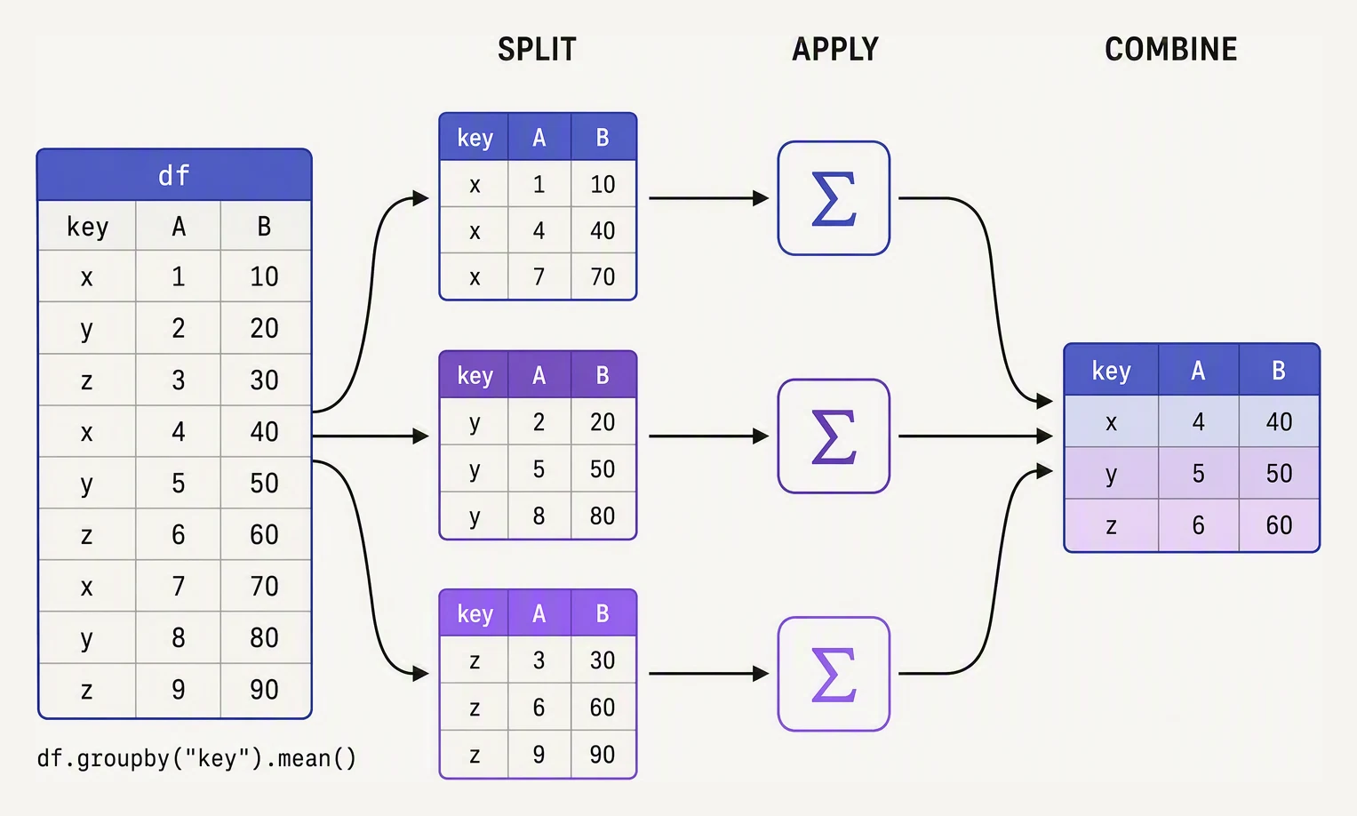
Split into groups, apply a reduction to each, combine the answers back.
df.groupby("user_id")["revenue"].sum() does three things:
- Split — divide the rows into groups by
user_id. Each unique value gets its own sub-DataFrame. - Apply — run the function (
sum) independently on each group’srevenuecolumn. - Combine — stitch the per-group results back into one Series indexed by
user_id.
That’s it. Every groupby fits this template. That’s why “per-user total” and “per-country average” have identical syntax; the only thing that changes is which column decides the groups.
Watch a groupby split into groups, apply a function, and collapse
groupby is really three moves. Split the rows into groups by a key, apply a function to each group, then combine the results into one row per group. Pick a key and a function, then Step or Run the three stages below.
region| region | product | sales |
|---|---|---|
| East | Widget | 120 |
| West | Gadget | 90 |
| East | Gadget | 60 |
| North | Widget | 200 |
| West | Gizmo | 150 |
| East | Widget | 80 |
| North | Gizmo | 110 |
| West | Gadget | 70 |
region → 3 groups8 rows collapse to 3, one per distinct region.df.groupby("region")["sales"].sum()| region | sales |
|---|---|
| East | 260 |
| West | 310 |
| North | 310 |
The setup: an events table
import pandas as pd

events = pd.DataFrame({
    "user_id":  ["u-1","u-2","u-1","u-3","u-2","u-1","u-3","u-1"],
    "event":    ["view","view","purchase","view","purchase","purchase","view","purchase"],
    "ts":       pd.to_datetime([
        "2026-05-20 09:00","2026-05-20 09:10","2026-05-20 09:15",
        "2026-05-21 10:00","2026-05-21 10:05","2026-05-21 11:30",
        "2026-05-22 08:00","2026-05-22 14:20",
    ]),
    "revenue":  [0.0, 0.0, 24.99, 0.0, 49.99, 14.50, 0.0, 99.00],
    "country":  ["IN","US","IN","DE","US","IN","DE","IN"],
})
print(events)
user_id event ts revenue country
0 u-1 view 2026-05-20 09:00:00 0.00 IN
1 u-2 view 2026-05-20 09:10:00 0.00 US
2 u-1 purchase 2026-05-20 09:15:00 24.99 IN
3 u-3 view 2026-05-21 10:00:00 0.00 DE
4 u-2 purchase 2026-05-21 10:05:00 49.99 US
5 u-1 purchase 2026-05-21 11:30:00 14.50 IN
6 u-3 view 2026-05-22 08:00:00 0.00 DE
7 u-1 purchase 2026-05-22 14:20:00 99.00 INA small event log. We’ll pull per-user, per-country, and per-day metrics from it.
One column, one aggregation
import pandas as pd

events = pd.DataFrame({
    "user_id":  ["u-1","u-2","u-1","u-3","u-2","u-1","u-3","u-1"],
    "revenue":  [0.0, 0.0, 24.99, 0.0, 49.99, 14.50, 0.0, 99.00],
})

# Total revenue per user
print(events.groupby("user_id")["revenue"].sum())
print()

# Average order value per user (just considering purchases > 0)
print(events[events["revenue"] > 0].groupby("user_id")["revenue"].mean().round(2))
user_id
u-1 138.49
u-2 49.99
u-3 0.00
Name: revenue, dtype: float64
user_id
u-1 46.16
u-2 49.99
Name: revenue, dtype: float64The result is a Series indexed by user_id.
Notice that the second call filtered to purchases first, so u-3 (zero purchases) drops out of the average entirely. Pass as_index=False to get a DataFrame with user_id as a regular column — handy when piping into a join.
Multiple aggregations with agg
You’ll usually want more than one number per group. The cleanest syntax is named aggregations:
import pandas as pd

events = pd.DataFrame({
    "user_id":  ["u-1","u-2","u-1","u-3","u-2","u-1","u-3","u-1"],
    "ts":       pd.to_datetime([
        "2026-05-20 09:00","2026-05-20 09:10","2026-05-20 09:15",
        "2026-05-21 10:00","2026-05-21 10:05","2026-05-21 11:30",
        "2026-05-22 08:00","2026-05-22 14:20",
    ]),
    "revenue":  [0.0, 0.0, 24.99, 0.0, 49.99, 14.50, 0.0, 99.00],
})

# Per-user metrics: total revenue, first order date, LTV (sum of purchases)
metrics = events.groupby("user_id").agg(
    total_revenue   = ("revenue", "sum"),
    first_seen      = ("ts",      "min"),
    last_seen       = ("ts",      "max"),
    event_count     = ("ts",      "count"),
    avg_revenue     = ("revenue", "mean"),
).round(2)

print(metrics)
total_revenue first_seen last_seen event_count avg_revenue
user_id
u-1 138.49 2026-05-20 09:00:00 2026-05-22 14:20:00 4 34.62
u-2 49.99 2026-05-20 09:10:00 2026-05-21 10:05:00 2 25.00
u-3 0.00 2026-05-21 10:00:00 2026-05-22 08:00:00 2 0.00The name=(column, func) syntax is the modern way. Each line names the output column and specifies
which input column and which aggregation to use. The result is a flat DataFrame — no hierarchical
column index to fight.
func can be one of these strings:
"sum""mean""min""max""count""nunique""first""last"
It can also be any callable.
Grouping by multiple columns
import pandas as pd

events = pd.DataFrame({
    "user_id":  ["u-1","u-2","u-1","u-3","u-2","u-1","u-3","u-1"],
    "country":  ["IN","US","IN","DE","US","IN","DE","IN"],
    "revenue":  [0.0, 0.0, 24.99, 0.0, 49.99, 14.50, 0.0, 99.00],
})

# Revenue by country, then by user
print(events.groupby(["country", "user_id"])["revenue"].sum())
country user_id
DE u-3 0.00
IN u-1 138.49
US u-2 49.99
Name: revenue, dtype: float64The result has a MultiIndex (country, user_id). Call .reset_index() to flatten it back into a
regular DataFrame with those as columns.
transform — broadcast back to original shape
agg collapses each group to a single row. transform instead returns a result the same shape
as the input. It broadcasts the per-group value to every row in that group — perfect for per-group
normalisation:
import pandas as pd

events = pd.DataFrame({
    "user_id":  ["u-1","u-2","u-1","u-3","u-2","u-1","u-3","u-1"],
    "revenue":  [0.0, 0.0, 24.99, 0.0, 49.99, 14.50, 0.0, 99.00],
})

# Add a column: how much THIS user has spent in total
events["user_total"] = events.groupby("user_id")["revenue"].transform("sum")

# What fraction of this user's total was this row?
events["share_of_user"] = (events["revenue"] / events["user_total"]).round(2).fillna(0)

print(events)
user_id revenue user_total share_of_user
0 u-1 0.00 138.49 0.00
1 u-2 0.00 49.99 0.00
2 u-1 24.99 138.49 0.18
3 u-3 0.00 0.00 0.00
4 u-2 49.99 49.99 1.00
5 u-1 14.50 138.49 0.10
6 u-3 0.00 0.00 0.00
7 u-1 99.00 138.49 0.71Every row kept its place, but now carries its user’s total (138.49 for all three u-1 rows) and its share of it (the 99.00 purchase is 0.71 of u-1’s spend).
transform is what you reach for when you want a per-group statistic right beside the original row
— “how far above this user’s average is this purchase?”, “rank within group”, and so on.
filter — keep or drop entire groups
filter runs a predicate on each group and keeps all rows of the groups that pass:
import pandas as pd

events = pd.DataFrame({
    "user_id":  ["u-1","u-2","u-1","u-3","u-2","u-1","u-3","u-1"],
    "revenue":  [0.0, 0.0, 24.99, 0.0, 49.99, 14.50, 0.0, 99.00],
})

# Only keep rows from users who spent more than $50 total
big_spenders = events.groupby("user_id").filter(
    lambda g: g["revenue"].sum() > 50
)
print(big_spenders)
user_id revenue
0 u-1 0.00
2 u-1 24.99
5 u-1 14.50
7 u-1 99.00Only u-1 cleared $50 total (138.49), so all four of its rows survive — including the two zero-revenue views.
That is the point of filter: a whole-group decision, all-or-nothing. (Don’t confuse it with
df.filter(...), which selects columns by name pattern.)
apply — the escape hatch (use sparingly)
apply runs any Python function on each group. It is flexible, but slow — pandas can’t vectorize
it.
Reach for it only when agg, transform, and built-ins genuinely can’t express what you need.
import pandas as pd

events = pd.DataFrame({
    "user_id":  ["u-1","u-2","u-1","u-3","u-2","u-1","u-3","u-1"],
    "revenue":  [0.0, 0.0, 24.99, 0.0, 49.99, 14.50, 0.0, 99.00],
})

# Top-2 purchases per user (something agg can't do directly)
top_per_user = (
    events
    .groupby("user_id")
    .apply(lambda g: g.nlargest(2, "revenue"), include_groups=False)
)
print(top_per_user)
revenue
user_id
u-1 7 99.00
2 24.99
u-2 4 49.99
1 0.00
u-3 3 0.00
6 0.00include_groups=False hands your function each group without its user_id column, and pandas puts
the key back in the index instead. Since pandas 3.0 that is the only behaviour (the key column is never
passed in), so writing it explicitly keeps the code identical on pandas 2.2 and 3.
Each user kept its two highest rows — a per-group top-N that agg (which collapses to one row)
simply cannot express. This is the legitimate use of the escape hatch.
A complete worked example — LTV per user
Here is how those pieces combine into something you would ship to a real BI dashboard:
import pandas as pd

events = pd.DataFrame({
    "user_id":  ["u-1","u-2","u-1","u-3","u-2","u-1","u-3","u-1","u-2"],
    "event":    ["view","view","purchase","view","purchase","purchase","view","purchase","purchase"],
    "ts":       pd.to_datetime([
        "2026-05-20","2026-05-20","2026-05-20","2026-05-21",
        "2026-05-21","2026-05-21","2026-05-22","2026-05-22","2026-05-23",
    ]),
    "revenue":  [0,0,24.99,0,49.99,14.50,0,99.00,29.00],
})

purchases = events[events["event"] == "purchase"]

ltv = purchases.groupby("user_id").agg(
    first_order_date = ("ts",      "min"),
    last_order_date  = ("ts",      "max"),
    order_count      = ("ts",      "count"),
    total_revenue    = ("revenue", "sum"),
    avg_order_value  = ("revenue", "mean"),
).round(2)

# Days between first and last order — "customer lifespan"
ltv["lifespan_days"] = (ltv["last_order_date"] - ltv["first_order_date"]).dt.days

print(ltv)
first_order_date last_order_date order_count total_revenue avg_order_value lifespan_days
user_id
u-1 2026-05-20 2026-05-22 3 138.49 46.16 2
u-2 2026-05-21 2026-05-23 2 78.99 39.50 2Filter to purchases, group by user, name five aggregates, then derive a sixth from two of them — one row per customer, every metric a BI team asks for.
(u-3, with no purchases, correctly never appears.)
In one breath
groupby is split–apply–combine: split rows by a key, apply a function per group, and combine
the results.
df.groupby("k")["v"].sum() gives one number per group. Named aggregations
agg(name=(col, func)) give several flat columns at once. Grouping by a list of keys produces a
MultiIndex.
The four verbs are:
aggcollapses each group to one row.transformbroadcasts the per-group value back to every original row (per-group normalisation/ranking).filterkeeps or drops whole groups by a predicate.applyis the slow, flexible escape hatch (per-group top-N).
Prefer the others over apply. The everyday output shape is one row per entity with aggregated metric
columns.
Practice
Quick check
groupby('u').agg('sum') and groupby('u').transform('sum')?total_revenue (sum) and n_orders (count) per user?city, date, temp_c. You want a new column temp_anomaly = each reading minus that city's mean temperature. Which approach is correct?A question to carry forward
groupby is enormously powerful, but notice its one hard limit: it only ever works within a single
table. Every metric we computed lived in the columns of events already.
Real questions rarely stay inside one table:
- Your orders sit in one place.
- Your customer names and countries are in another.
- Your events reference a
device_idwhose details live in a separate file.
To answer “revenue by country”, you first have to bring the country over from the customers table onto the orders.
That stitching-together of two tables on a shared key is merge — SQL joins, in pandas.
What are the four join flavours?
- inner
- left
- right
- outer
Why can an innocent-looking join silently double your row count and quietly inflate every total downstream? What single argument — validate — stops that from ever happening unnoticed?
Questions about this lesson
How does groupby work in Pandas?
groupby splits the DataFrame into groups by one or more key columns, applies a function to each group (like sum, mean, or a custom aggregation), and combines the results — the split-apply-combine pattern. The keys become the result's index by default.
What's the difference between agg, transform, and apply?
agg returns one summary row per group; transform returns a result the same shape as the input, ideal for group-wise normalisation; apply is the most flexible but slowest, accepting any per-group function. Prefer agg or transform when you can.
How do I keep the group keys as columns instead of the index?
Pass as_index=False to groupby, or call .reset_index() on the result. By default the group keys become the index, and reset_index() turns them back into regular columns.
Practice this in an interview
All questionsPass a dictionary to agg() mapping each column to one or more functions, or use named aggregations with the keyword-argument form (pandas 0.25+) to control output column names directly. Both approaches avoid chained GroupBy calls and produce a clean, single-pass result.
Grouping on multiple keys produces a MultiIndex on the result by default. You can suppress it with asindex=False or groupby(..., asindex=False), or reset it afterward with resetindex(). Stacking and unstacking let you pivot between long and wide forms once a MultiIndex exists.
GroupBy splits a DataFrame into subgroups by key, applies a function independently to each group, then combines the results back into a single object. Understanding which phase each method targets — agg collapses, transform preserves shape, filter removes entire groups — determines which API to reach for.
agg collapses each group into a single scalar, returning a result with one row per group. transform returns a Series or DataFrame with the same index as the original, broadcasting the group-level result back to every row — making it ideal for adding derived columns without a merge.