Method chaining — write transforms like an f-string
Chain DataFrame operations into one fluent pipeline. .pipe, .assign, .query — and the one place where breaking the chain still pays.
Written and reviewed by Shreyash Prashu Last reviewed
What you'll learn
- Why chaining beats intermediate-variable spaghetti
-
.assign,.query, and.pipe— the three chain-friendly verbs - The "f-string body" layout that makes long chains readable
- When NOT to chain (debugging, branching, side-effecting code)
Before you start
Look back at the closing thought from the time-series lesson. Every transformation we wrote across
this whole section had the same shape — read a file, filter rows, group, aggregate, reshape — and at
each step we either reassigned a throwaway variable (df = df.something(), again and again) or
buried one call inside another. It runs. But it reads like a pile of statements, not a single
thought.
Open any analytical script that has grown over a few months and you’ll see what that costs. The same
shape every time: a dozen intermediate DataFrames — df, df2, df_clean, df_clean_2,
df_final, df_final_v2 — each one used exactly once, none of the names meaning anything. The flow
of the transformation is buried in the assignments.
There is a cleaner way. Method chaining means calling each method directly on the return value of
the one before, so df.step1().step2().step3() becomes a single expression that reads top to bottom
like a recipe. Let’s take an ordinary script and watch it collapse.
The “before” — intermediate-variable style
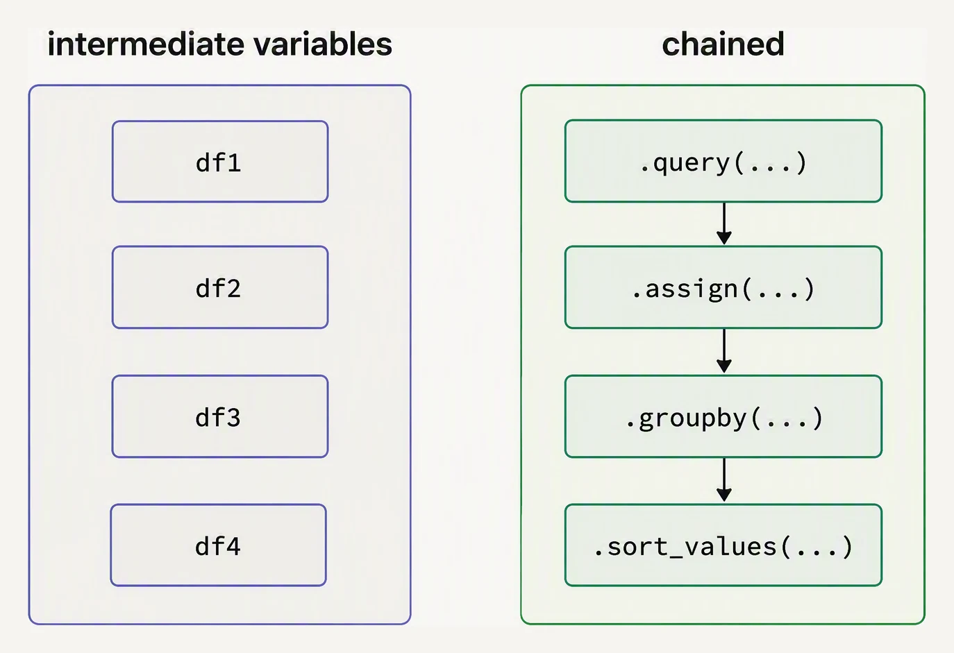
A chain reads top to bottom as one sentence. No intermediate names to keep straight.
Here is a typical orders-analysis script. Every step gets its own variable.
import pandas as pd

orders = pd.DataFrame({
    "order_id":   ["o-1","o-2","o-3","o-4","o-5","o-6","o-7","o-8"],
    "customer":   ["alice","bob","alice","carol","bob","alice","carol","dave"],
    "amount":     [120.0, 45.50, 0.0, 89.99, 210.0, 15.0, 67.5, 330.0],
    "status":     ["paid","paid","cancelled","paid","paid","refunded","paid","paid"],
    "country":    ["IN","US","IN","DE","US","IN","DE","US"],
})

# Step 1: filter to paid orders only
paid = orders[orders["status"] == "paid"]

# Step 2: drop the status column (now all the same)
paid_2 = paid.drop(columns=["status"])

# Step 3: add a 10% tax column
paid_3 = paid_2.copy()
paid_3["tax"] = paid_3["amount"] * 0.10

# Step 4: keep only US and IN
paid_4 = paid_3[paid_3["country"].isin(["US","IN"])]

# Step 5: per-customer totals
totals = paid_4.groupby("customer", as_index=False).agg(
    n_orders=("order_id","count"),
    revenue=("amount","sum"),
    tax=("tax","sum"),
)

# Step 6: sort, top 3
result = totals.sort_values("revenue", ascending=False).head(3)
print(result)
customer n_orders revenue tax
2 dave 1 330.0 33.00
1 bob 2 255.5 25.55
0 alice 1 120.0 12.00Six steps, four throwaway variables. Reading it top to bottom, you have to track the suffixes —
paid, paid_2, paid_3, paid_4 — just to know which one feeds the next. Rename one and you have
to chase it through the whole script.
The “after” — chained style
Same transformation. One expression.
result = (
    orders
    .query("status == 'paid'")
    .drop(columns=["status"])
    .assign(tax=lambda d: d["amount"] * 0.10)
    .query("country in ['US','IN']")
    .groupby("customer", as_index=False)
    .agg(n_orders=("order_id","count"),
         revenue=("amount","sum"),
         tax=("tax","sum"))
    .sort_values("revenue", ascending=False)
    .head(3)
)
print(result)
customer n_orders revenue tax
2 dave 1 330.0 33.00
1 bob 2 255.5 25.55
0 alice 1 120.0 12.00Identical result — same three customers, same numbers — but no intermediate names. The pipeline now
reads as six verbs in order: filter, drop, add a column, filter again, aggregate, sort. The outer
parentheses are the whole trick: once you wrap the expression in ( ... ), you can break the line
after every . and Python stays happy.
The three chain-friendly verbs
A method only belongs in a chain if it returns a DataFrame — otherwise the next .method has
nothing to call on. Three verbs cover almost everything you’ll want to do mid-chain.
.assign — add or replace columns
The everyday df["new_col"] = ... mutates in place and returns None, which snaps a chain. .assign
instead returns a new DataFrame with the column added, so it slots right in.
cart = pd.DataFrame({
    "amount":   [120.0, 45.50, 89.99, 210.0],
    "shipping": [9.99, 4.99, 4.99, 0.0],
})

out = (
    cart
    .assign(
        subtotal = lambda d: d["amount"] + d["shipping"],
        tax      = lambda d: d["subtotal"] * 0.10,
        total    = lambda d: d["subtotal"] + d["tax"],
    )
    .round(2)
)
print(out) amount shipping subtotal tax total
0 120.00 9.99 129.99 13.00 142.99
1 45.50 4.99 50.49 5.05 55.54
2 89.99 4.99 94.98 9.50 104.48
3 210.00 0.00 210.00 21.00 231.00It works, and that is the point. The lambda d: ... form is what makes .assign powerful: each
lambda receives the DataFrame as it exists after every earlier keyword in the same call, so later
columns can lean on ones created a line above. (Scalar values like assign(col=5) are evaluated
immediately and don’t get this in-flight view — only the lambda form does.) One call, a whole ladder
of dependent columns.
.query — filter with a string expression
The standard df[df["a"] > 5] writes df twice — once to index, once for the condition. .query
says the same thing once.
# These two are equivalent
orders[orders["country"].isin(["US","IN"]) & (orders["amount"] > 50)]
orders.query("country in ['US','IN'] and amount > 50")
On large DataFrames .query is also a little faster, because it hands the expression to a specialized
evaluation engine instead of building intermediate boolean arrays.
.pipe — drop in your own function
Sometimes the step you need isn’t a built-in DataFrame method at all — it’s a custom cleaning
routine, a domain-specific feature engineer, a call into a sibling library. .pipe(fn) calls
fn(df) and hands back the result, so your own function joins the chain as just another verb.
def add_revenue_tier(df, low=50, high=200):
    """Bucket each order into low / medium / high."""
    bins = [-1, low, high, float("inf")]
    labels = ["low", "medium", "high"]
    return df.assign(tier=pd.cut(df["amount"], bins=bins, labels=labels))

orders = pd.DataFrame({
    "order_id": ["o-1","o-2","o-3","o-4","o-5"],
    "amount":   [25.0, 89.99, 210.0, 45.0, 330.0],
})

result = (
    orders
    .query("amount > 0")
    .pipe(add_revenue_tier, low=50, high=200)
    .sort_values("amount")
)
print(result)
order_id amount tier
0 o-1 25.00 low
3 o-4 45.00 low
1 o-2 89.99 medium
2 o-3 210.00 high
4 o-5 330.00 highAny extra keyword arguments after the function are forwarded — so add_revenue_tier is called as
add_revenue_tier(df, low=50, high=200). That’s how you keep heavy custom logic out of the chain
body while still threading it through the flow.
The “f-string body” layout
For any chain longer than two or three steps, one layout makes the difference between readable and cryptic — the same shape Python’s multi-line f-strings use. Open paren on its own line, one method per line, closing paren on its own line.
result = (
    df
    .verb_one(...)
    .verb_two(...)
    .verb_three(...)
)
Every line starts with a ., every step is visually a row. Diffs stay clean too: inserting a step is
a one-line addition, not a rewrite of the surrounding statements.
When NOT to chain
Chaining is a style, not a vow. Break the chain when:
- You need to debug step by step. You can’t set a breakpoint between two methods inside one expression. When a transform misbehaves, pull it apart, inspect the in-flight DataFrame at each step, fix it, then re-collapse the chain once it works.
- The same intermediate is reused. If one stage feeds both a model and a chart, it has earned a name — give it one.
- A step has side effects — writing to disk, logging, raising on a condition. Side effects belong in named functions, not buried inline.
- The chain crosses eight to ten steps. Past that, split it into two chains joined by a named
intermediate that says what the data is at that point (
paid_orders_with_tax, notdf_4).
A good test: would a colleague reading this in six months thank you for the chain, or curse you? If it reads like a clean recipe, ship it. If it reads like a riddle, name the stages.
In one breath
Method chaining replaces a pile of single-use intermediate DataFrames with one expression that reads
top to bottom like a recipe — wrap it in parentheses, one verb per line. Three verbs keep the chain
alive because each returns a DataFrame: .assign adds columns (use the lambda d: ... form so later
columns can lean on earlier ones), .query filters with a string instead of repeating df, and
.pipe drops your own function in as just another step. Break the chain — and use a named
intermediate — when you need to debug, reuse a stage, run a side effect, or once it grows past
roughly ten steps.
Practice
Quick check
df.assign(new=df['a']*2) work inside a chain but df['new'] = df['a']*2 doesn't?.pipe(my_func, threshold=10) do?A question to carry forward
The chain reads beautifully — but trace what it actually does at runtime. .query returns a new
DataFrame. .assign returns another. .groupby().agg() returns another. Every verb in the pipeline
allocates a fresh copy of the data. On eight rows that’s free. On eight million rows, each of those
copies is real memory, and a chain that looks elegant can quietly hold several full versions of your
table at once.
So before we worry about speed, we have to worry about size. How much memory is a DataFrame
actually using — and why does a 600 MB CSV sometimes balloon to 8 GB the moment you load it? The next
lesson is memory: how to measure the true footprint with info(memory_usage='deep'), and how
downcasting, categoricals, and a smarter read_csv routinely cut it by 5x or more — with no loss of
information at all.
Practice this in an interview
All questionsMethod chaining applies a sequence of transformations in a single expression without intermediate variables, improving readability and reducing accidental mutation. pipe() inserts any callable — including custom functions and sklearn transformers — into the chain, keeping data flow linear even when a function takes the DataFrame as a non-first argument.
GroupBy splits a DataFrame into subgroups by key, applies a function independently to each group, then combines the results back into a single object. Understanding which phase each method targets — agg collapses, transform preserves shape, filter removes entire groups — determines which API to reach for.
agg collapses each group into a single scalar, returning a result with one row per group. transform returns a Series or DataFrame with the same index as the original, broadcasting the group-level result back to every row — making it ideal for adding derived columns without a merge.
Every core SQL clause — SELECT, WHERE, GROUP BY, HAVING, JOIN, ORDER BY, LIMIT — has a direct pandas equivalent, but SQL executes inside a database engine with optimized query planning and disk-backed storage, while pandas requires all data to fit in RAM. Use SQL for large persistent datasets and pandas for in-memory transformation, feature engineering, and integration with the Python ML ecosystem.