Boolean masks
Comparison ops, mask combinators, np.where — the filter-and-modify toolkit that powers every Pandas query under the hood.
Written and reviewed by Shreyash Prashu Last reviewed
What you'll learn
- Comparison ops produce boolean arrays that index like masks
- Combining masks with
&,|,~— and why you MUST parenthesize -
np.wherefor both filtering and conditional assignment -
np.any,np.allfor checking conditions across axes
Before you start
The last lesson kept reaching for a tool it never named. true == c built a boolean array;
(pred == true).mean() poured booleans into a mean to count the Trues; pred[mask] lifted out a
scattered subset. That tool — the boolean mask — is the single most-used pattern in all of data
work, and most of it is one sentence: find the elements that match a condition, then do something
to them. Boolean masking is how NumPy does that with no loop, and once it clicks, every Pandas
df[df['col'] > 5] query stops feeling like magic — it is exactly this, one layer down.
Comparisons return boolean arrays
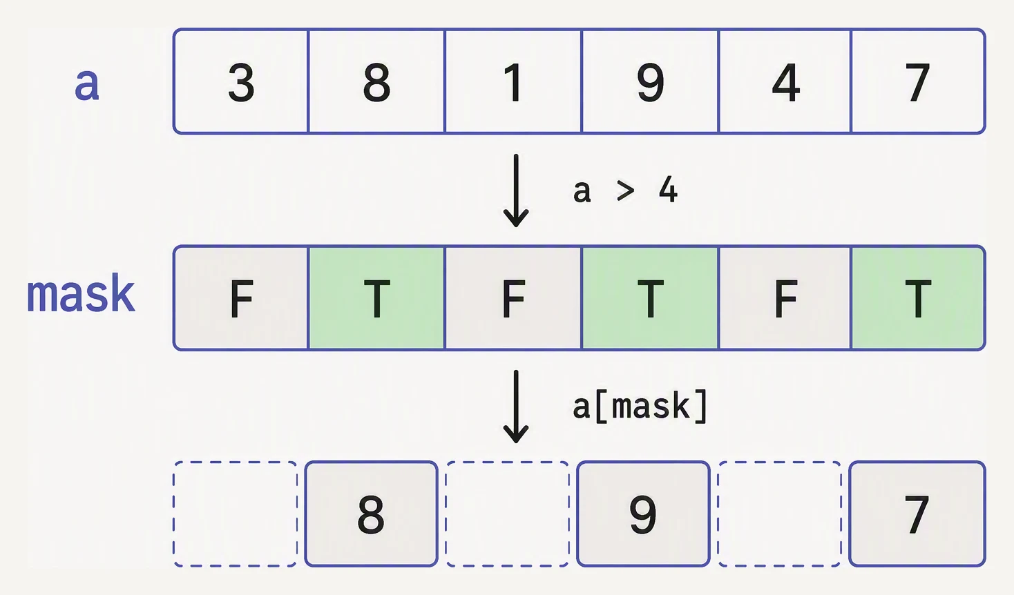
The comparison builds a mask. The mask does the selecting.
Every comparison operator (==, !=, <, >, <=, >=) is a ufunc: it broadcasts and returns a
boolean array of the same shape.
import numpy as np

# Daily closing prices for a stock — 10 trading days.
prices = np.array([102.5, 101.0, 99.8, 105.3, 110.2,
                   108.4, 95.0, 97.5, 103.1, 109.0])

# Which days closed above 100?
above_100 = prices > 100
print("mask  :", above_100)
print("count :", above_100.sum())   # True counts as 1

# Pick those prices.
print("values:", prices[above_100])

# Or do it inline (most common style).
print("inline:", prices[prices > 100])
mask : [ True True False True True True False False True True]
count : 7
values: [102.5 101. 105.3 110.2 108.4 103.1 109. ]
inline: [102.5 101. 105.3 110.2 108.4 103.1 109. ]The boolean mask (a same-shape array of True/False) tells NumPy which elements to keep; indexing
with it returns a 1-D array of the True-valued elements — and feeding it to .sum() counts them
(True = 1). This is the most-used pattern in NumPy, full stop.
Pick a condition — watch the mask form
A boolean mask is just an array of True/False with the same shape as the data. Indexing with it keeps only the True positions.
[T, F, T, F, F, F, T, T, T, F, F, T, T, T, F, T][4, 2, 7, 1, 6, 3, 5, 8, 2]Combining masks — &, |, ~ (and parens!)
You combine boolean arrays with bitwise operators, not Python’s and/or/not. And you
must wrap each comparison in parentheses, because the bitwise operators bind tighter than <
and >.
import numpy as np

prices = np.array([102.5, 101.0, 99.8, 105.3, 110.2,
                   108.4, 95.0, 97.5, 103.1, 109.0])
volume = np.array([1000, 1200, 800, 2500, 3000,
                   2800, 500, 700, 2100, 2900])

# Days that were both "high price" AND "high volume."
mask = (prices > 105) & (volume > 2000)
print("high price & high volume:")
print("  prices:", prices[mask])
print("  volume:", volume[mask])

# Days that were either low price OR low volume (anomalies).
low = (prices < 100) | (volume < 1000)
print("\nlow either way:", prices[low])

# Invert a mask: NOT.
not_low = ~low
print("not low      :", prices[not_low])
high price & high volume:
prices: [105.3 110.2 108.4 109. ]
volume: [2500 3000 2800 2900]
low either way: [99.8 95. 97.5]
not low : [102.5 101. 105.3 110.2 108.4 103.1 109. ]If you forget and reach for Python’s and, you will get
"truth value of an array with more than one element is ambiguous" — NumPy telling you to use &.
A real filter — outlier detection
import numpy as np

# Sensor readings (°C). The sensor occasionally spikes — outliers.
rng = np.random.default_rng(0)
readings = 20 + 2 * rng.standard_normal(50)
readings[[7, 23, 41]] = [80, -30, 95]   # spike anomalies

# Define outliers as "more than 3 std from the mean."
mean = readings.mean()
std  = readings.std()
outlier = np.abs(readings - mean) > 3 * std

print("total samples :", len(readings))
print("outliers found:", outlier.sum())
print("outlier values:", readings[outlier])

# Clean array: keep only the non-outliers.
clean = readings[~outlier]
print("clean mean    :", clean.mean().round(2),
      "(was", round(mean, 2), ")")
total samples : 50
outliers found: 3
outlier values: [ 80. -30. 95.]
clean mean : 20.15 (was 21.85 )The mask |readings − mean| > 3·std flagged exactly the three injected spikes; dropping them with
~outlier pulls the mean from a corrupted 21.85 back to the honest 20.15. Three-sigma filtering is
the simplest, most common cleanup recipe in any quant or sensor pipeline.
np.where — vectorized if/else
np.where(cond, a, b) is the vectorized ternary: where the condition is True, take from a; where
False, take from b.
import numpy as np

# ML label encoding: turn raw scores into binary labels.
scores = np.array([0.2, 0.6, 0.9, 0.4, 0.1, 0.75, 0.55])
labels = np.where(scores >= 0.5, 1, 0)
print("labels :", labels)

# Clip negative returns to zero (e.g., for downside-only stats).
returns = np.array([0.02, -0.03, 0.01, -0.05, 0.04, -0.01])
downside = np.where(returns < 0, returns, 0)
print("downside:", downside)

# More elaborate: tag by magnitude.
tagged = np.where(np.abs(returns) > 0.03, "big", "small")
print("tags    :", tagged)
labels : [0 1 1 0 0 1 1]
downside: [ 0. -0.03 0. -0.05 0. -0.01]
tags : ['small' 'small' 'small' 'big' 'big' 'small']Called with a single argument — np.where(mask) — it returns the indices where the mask is
True, the inverse of boolean indexing: positions, not values.
import numpy as np

prices = np.array([102, 101, 99, 105, 110, 108, 95, 97, 103, 109])

# Indices of days that closed above 105.
idx = np.where(prices > 105)
print("indices  :", idx)        # tuple — (array([4, 5, 9]),)
print("indices  :", idx[0])     # just the array
print("at those :", prices[idx])
indices : (array([4, 5, 9]),)
indices : [4 5 9]
at those : [110 108 109]The tuple wrapping looks awkward, but it is consistent with multi-axis where, which returns one
index array per axis.
np.any and np.all — reductions over booleans
When you need “is any element True?” or “are all True?”, these are the reductions — and like
every reduction they take an axis.
import numpy as np

# A batch of 5 samples × 4 features. NaN means "missing measurement."
X = np.array([
    [1.0, 2.0, 3.0, 4.0],
    [1.0, np.nan, 3.0, 4.0],
    [1.0, 2.0, 3.0, 4.0],
    [np.nan, np.nan, 3.0, 4.0],
    [1.0, 2.0, 3.0, 4.0],
])

# Mark which samples have any missing data.
has_nan = np.isnan(X).any(axis=1)
print("samples with NaN:", has_nan)

# Mark features with NO missing data across all samples.
fully_observed = ~np.isnan(X).any(axis=0)
print("clean features  :", fully_observed)

# Quick sanity: is *every* sample missing at least one value?
print("all rows bad?   :", has_nan.all())
samples with NaN: [False True False True False]
clean features : [False False True True]
all rows bad? : Falseisnan(X).any(axis=1) reads “for each row, does any column hold a NaN?” — rows 1 and 3 do.
Collapsing along axis=0 instead asks it per column: features 2 and 3 are fully observed. This is
the backbone of any data-quality report.
Modifying via masks
Anything a mask can select, it can also assign — the way you “fix” or “clamp” values.
import numpy as np

# A feature column with sentinel values (-999 = missing) we need to
# replace before training.
feature = np.array([1.2, 0.5, -999, 3.4, -999, 2.1, 0.8, -999, 4.0])

# Replace sentinels with the median of the valid values.
valid = feature[feature != -999]
feature[feature == -999] = np.median(valid)
print("fixed:", feature)
fixed: [1.2 0.5 1.65 3.4 1.65 2.1 0.8 1.65 4. ]The three -999 sentinels became 1.65 — the median of the six valid readings — in one masked
assignment, no loop.
In one breath
A comparison (prices > 100) returns a same-shape boolean mask; indexing with it keeps the
True elements and .sum() counts them. Combine masks with bitwise &/|/~ — never Python
and/or — and always parenthesize each comparison ((a > 1) & (b < 2)), because & binds
tighter than </>. np.where(cond, a, b) is the vectorized if/else (label encoding, clipping);
np.where(mask) alone returns the True indices. np.any/np.all reduce booleans along an
axis (per-row/per-column NaN checks). And masks assign as well as select — arr[arr == -999] = median fixes sentinels in one line. This is the query language under every Pandas/SQL filter.
Practice
Quick check
arr to elements where x is positive AND less than 10?arr[arr > 0] and np.where(arr > 0)?X of shape (n_samples, n_features). How do you find samples (rows) that contain any NaN?A question to carry forward
Step back and look at everything the Vectorization chapter taught — ufuncs, broadcasting, aggregations, and now masks. Every one treats an array as a bag of independent numbers: compare each, transform each, reduce each, filter each. Position barely matters; element 5 never talks to element 50.
But the operation at the dead centre of machine learning does the opposite. It mixes elements —
every output number is woven from a whole row and a whole column at once. A neural-net layer, a
linear-regression fit, a PCA, an attention score: all of them are one operation, and it is not
element-wise. The next chapter opens on it. What is matrix multiplication in NumPy — the @
operator, np.dot, np.matmul — what is the shape rule that makes (64, 784) @ (784, 128)
collapse to (64, 128), and why is that single rule the engine under every dense layer ever
written?
Practice this in an interview
All questionsBoolean indexing filters a DataFrame by passing a boolean Series or array of the same length as the index. Common pitfalls include using Python's and/or instead of &/| and forgetting to wrap compound conditions in parentheses, both of which raise errors or produce wrong results.
Vectorized pandas and NumPy operations operate on entire arrays in compiled C/Fortran code and should always be your first choice. apply runs a Python function row- or column-wise in a Python loop, map transforms a single Series element-by-element, and applymap (DataFrame.map in pandas 2.1+) applies a function to every scalar — all three are orders of magnitude slower than vectorized equivalents.
duplicated() returns a boolean mask of rows that are duplicates of an earlier row; dropduplicates() removes them. Both accept a subset parameter to restrict comparison to specific columns and a keep parameter ('first', 'last', or False) to control which instance is retained or whether all copies are dropped.
Every core SQL clause — SELECT, WHERE, GROUP BY, HAVING, JOIN, ORDER BY, LIMIT — has a direct pandas equivalent, but SQL executes inside a database engine with optimized query planning and disk-backed storage, while pandas requires all data to fit in RAM. Use SQL for large persistent datasets and pandas for in-memory transformation, feature engineering, and integration with the Python ML ecosystem.