Universal functions (ufuncs)
Element-wise operations that run in C, beat Python loops by 100×, and accept out= and where= for in-place magic.
Written and reviewed by Shreyash Prashu Last reviewed
What you'll learn
- What makes a function a ufunc and why it's fast
- The arithmetic, trigonometric, exponential, and comparison ufuncs you'll use
- The
out=argument to avoid temporary allocations - The
where=argument for conditional computation
Before you start
The last lesson named this machinery without opening it. Broadcasting decided the shape of
X - mean and col * row; the thing that actually computed each output number — element by
element, in C, with no Python loop — is a ufunc, a “universal function.” Every +, -,
np.exp, np.sin you have ever typed is one, and they are the reason NumPy is fast. This lesson
opens the box: what makes a ufunc quick, and the controls — out=, where=, and .reduce — that
turn it from a convenience into a precision tool.
Ufuncs are why your code runs
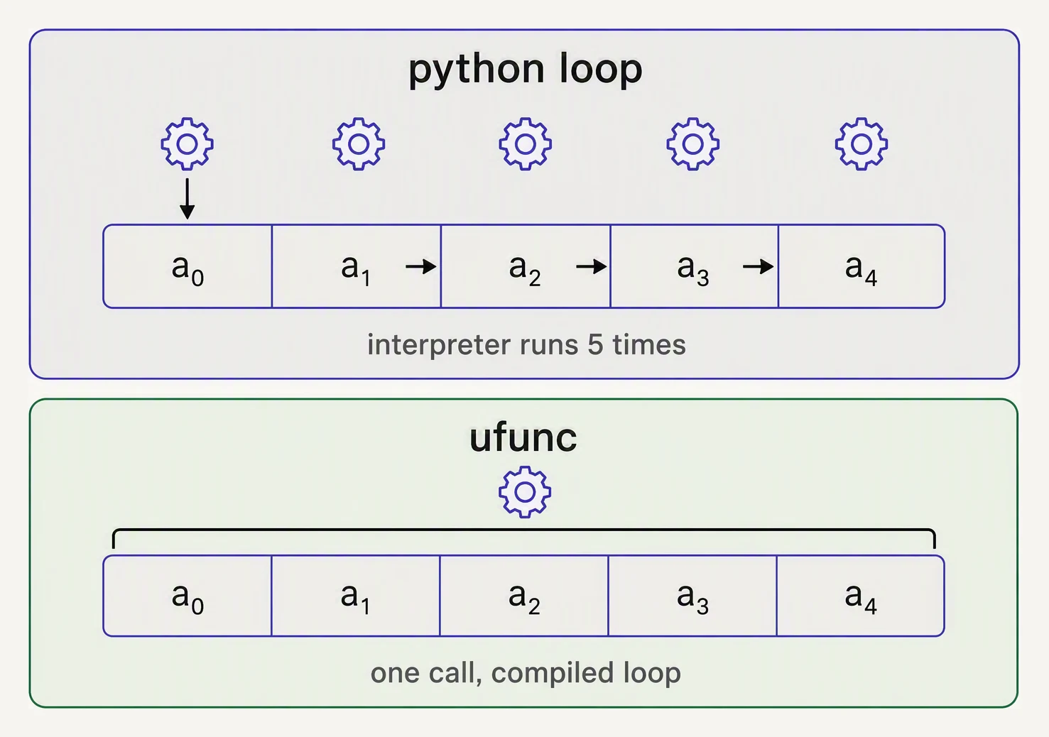
Same result. One pays the interpreter per element; the other doesn’t.
When you write a + b, you are calling np.add(a, b). That call runs a tight C loop with no
Python-interpreter overhead per element. The same loop written in Python is 50–200× slower — here,
computing the log-returns of a million-tick price series:
import numpy as np
import time

# Stock prices for 1 million ticks — a geometric random walk, so prices stay positive.
rng = np.random.default_rng(0)
p = 100 * np.exp(np.cumsum(rng.standard_normal(1_000_000) * 0.001))

# Log-returns: log(p[t]) - log(p[t-1])
# Vectorized: one ufunc call.
t0 = time.perf_counter()
log_p = np.log(p)
returns_vec = log_p[1:] - log_p[:-1]
t_vec = time.perf_counter() - t0

# Pure-Python loop equivalent.
p_list = p.tolist()
t0 = time.perf_counter()
returns_loop = [np.log(p_list[i]) - np.log(p_list[i-1])
                for i in range(1, len(p_list))]
t_loop = time.perf_counter() - t0

print(f"vectorized: {t_vec*1000:7.1f} ms")
print(f"loop      : {t_loop*1000:7.1f} ms")
print(f"speedup   : {t_loop/t_vec:7.1f}x")
vectorized: 2.9 ms
loop : 674.8 ms
speedup : 233.7x(Absolute milliseconds vary by machine; the two-to-three-orders-of-magnitude ratio is the invariant.) Computing log-returns is something you do a hundred times in finance code — the vectorized form is one line and hundreds of times faster.
The ufuncs you’ll use weekly
Arithmetic        +  -  *  /  //  %  **  np.add  np.subtract …
Negation          -arr  np.negative(arr)
Absolute          np.abs(arr)
Exponential/log   np.exp  np.log  np.log2  np.log10  np.log1p
Powers / roots    np.sqrt  np.cbrt  np.power(a, b)
Trig              np.sin  np.cos  np.tan  np.arcsin  np.arctan2
Hyperbolic        np.sinh  np.cosh  np.tanh
Rounding          np.round  np.floor  np.ceil  np.trunc
Comparison        ==  !=  <  >  np.maximum  np.minimum
Logical           np.logical_and  np.logical_or  np.logical_not
Bitwise           &  |  ^  ~  (on integer arrays)
These all return new arrays of the same shape. Two that trip people up:
np.maximum(a, b)is element-wise max of two arrays — different fromnp.max(a), which reduces one array to a single value.np.log1p(x)computeslog(1 + x)accurately for smallx— the numerical-stability fix from earlier, where1 + xwould otherwise round away.
A real ML feature transform
A common preprocessing step: apply log(1 + x) to a heavy-tailed feature to pull its long tail in
and make it more Gaussian.
import numpy as np

# Simulated user "purchase count" — heavy-tailed, mostly small, occasional whale.
rng = np.random.default_rng(1)
counts = rng.exponential(scale=20, size=10).round().astype(int)
print("raw counts :", counts)
print("mean       :", counts.mean().round(2),
      "max        :", counts.max())

# log1p flattens the long tail.
transformed = np.log1p(counts)
print("log1p      :", transformed.round(3))
print("mean       :", transformed.mean().round(2),
      "max        :", transformed.max().round(2))
raw counts : [ 21 6 108 7 2 36 10 11 1 15]
mean : 21.7 max : 108
log1p : [3.091 1.946 4.691 2.079 1.099 3.611 2.398 2.485 0.693 2.773]
mean : 2.49 max : 4.69The raw counts span 1 to 108 with a lone whale at 108; after log1p, everything sits between 0.69
and 4.69. The mean and max are now close together, so a model’s gradient won’t be hijacked by a few
extreme rows.
The out= argument — avoid allocations
Every a + b allocates a fresh array for the result. For large arrays in tight loops, that
allocation is the bottleneck. Pass out= to write into an existing buffer instead.
import numpy as np

a = np.arange(1_000_000, dtype=np.float64)
b = np.arange(1_000_000, dtype=np.float64) * 2

# Pre-allocate the result buffer once.
buf = np.empty_like(a)

# Reuse it on every operation — no per-call allocation.
np.add(a, b, out=buf)
print("buf[:5] :", buf[:5])

np.multiply(a, b, out=buf)
print("buf[:5] :", buf[:5])

# Compare with the allocating form:
result = a + b      # allocates a new million-element array.
print("equal   :", np.array_equal(buf, a * b))
buf[:5] : [ 0. 3. 6. 9. 12.]
buf[:5] : [ 0. 2. 8. 18. 32.]
equal : TrueIn production data pipelines and ML training loops, out= is the difference between a hot loop and
a memory-thrashing one.
The where= argument — conditional ufuncs
where=mask runs the ufunc only where the mask is True, leaving the rest untouched.
import numpy as np

# Pixel values, but some pixels (255) are saturated and we want to leave them alone
# while halving the brightness of the rest.
img = np.array([10, 100, 255, 50, 255, 200], dtype=np.uint8)
out = img.copy()

# Only divide the non-saturated pixels.
mask = img != 255
np.floor_divide(img, 2, out=out, where=mask)

print("input :", img)
print("output:", out)   # saturated 255s preserved, others halved.
input : [ 10 100 255 50 255 200]
output: [ 5 50 255 25 255 100]The two 255s pass through untouched while everything else is halved — in a single call, with no
boolean-copy step. That makes where= more efficient than first doing arr[mask] = ....
Ufunc reductions and accumulations
Every ufunc carries .reduce, .accumulate, and .outer methods. You will not reach for these
daily, but they reveal what the everyday functions really are.
import numpy as np

x = np.array([1, 2, 3, 4, 5])

# .reduce — apply the op across an axis (here: sum)
print("add.reduce       :", np.add.reduce(x))      # 15

# .accumulate — running totals
print("add.accumulate   :", np.add.accumulate(x))  # [1, 3, 6, 10, 15]

# .outer — full pairwise table
print("multiply.outer   :")
print(np.multiply.outer(x, x))   # the multiplication table
add.reduce : 15
add.accumulate : [ 1 3 6 10 15]
multiply.outer :
[[ 1 2 3 4 5]
[ 2 4 6 8 10]
[ 3 6 9 12 15]
[ 4 8 12 16 20]
[ 5 10 15 20 25]]np.add.reduce(arr) is exactly arr.sum(); np.multiply.accumulate(arr) is np.cumprod. The
everyday functions are these primitives in disguise.
In one breath
A ufunc (+, np.exp, np.maximum, …) applies an operation element-wise in C, the engine
behind NumPy’s 50–200× edge over Python loops (the log-returns demo: ~234× here). Broadcasting is
just how a ufunc lines up differently-shaped inputs. Reach for np.maximum(a, b) (two-array max,
not np.max’s reduction) and np.log1p/np.expm1 (numerically stable near zero). Two power
controls: out= writes into a pre-allocated buffer to skip per-call allocation (a += b is
out=a, but it won’t upcast — beware small-int overflow), and where=mask computes only on
the True elements. And every ufunc’s .reduce/.accumulate/.outer are the primitives behind
sum, cumprod, and outer products.
Practice
Quick check
np.max(arr) and np.maximum(a, b)?np.add(a, b, out=buf) matter for performance?np.log1p(x) instead of np.log(1 + x)?A question to carry forward
That last section quietly crossed a line. Every ufunc until then took an array and returned an
array of the same shape — element in, element out. But .reduce did the opposite: it
collapsed the whole array down to a single number (np.add.reduce([1,2,3,4,5]) = 15). That is
a different kind of operation — a reduction — and it is how you turn a million prices into one
mean, a feature matrix into a per-column standard deviation, a row of logits into one predicted
class.
So the next lesson is the toolbox of aggregations: sum, mean, std, min, argmax,
percentile. They are easy to name and easy to misuse, because they all hinge on one argument that
decides which axis collapses and what shape survives — axis. What exactly does axis=0
versus axis=1 do to an array, and why is keepdims=True the fix you’ll reach for again and
again?
Practice this in an interview
All questionsNumPy operations execute compiled C code over contiguous memory blocks in a single call, while a Python loop incurs interpreter overhead and dynamic type checks on every element. Vectorization means expressing an operation over an entire array at once so the hot path never re-enters the Python interpreter.
Vectorized pandas and NumPy operations operate on entire arrays in compiled C/Fortran code and should always be your first choice. apply runs a Python function row- or column-wise in a Python loop, map transforms a single Series element-by-element, and applymap (DataFrame.map in pandas 2.1+) applies a function to every scalar — all three are orders of magnitude slower than vectorized equivalents.
Python lists are heterogeneous, pointer-based, and general-purpose. NumPy arrays are homogeneous, stored as contiguous typed memory, and support vectorised operations that run at C speed. For numerical work on more than a few hundred elements, NumPy is almost always faster and more memory-efficient.
Python sets support union, intersection, difference, and symmetric difference as both operators and methods, all running in O(min(m,n)) to O(m+n) time. They are useful for deduplication, membership testing in large collections, and computing overlaps between datasets — operations that would be expensive with lists.