Creating arrays
zeros, ones, arange, linspace, random — the constructors you'll reach for every day, and when to use which.
Written and reviewed by Shreyash Prashu Last reviewed
What you'll learn
- The standard "shape-first" constructors — zeros, ones, full, empty
- The difference between arange (step) and linspace (count)
- Why
np.emptyis faster but dangerous - Random arrays for weights, simulations, and test data
Before you start
The last lesson left you typing arrays out by hand — np.array([4.5, 1.2, ...]) — and then
admitted you will almost never do that in real code. You don’t have the numbers; you have a
shape you want filled. A placeholder for 128 embeddings. A bias vector of ones. A range of
x-values for a plot. Random weights for an untrained model. This lesson is the toolbox of
constructors that conjure an array from a shape alone — six of them cover about 95% of what you
will ever reach for.
Filled arrays — zeros, ones, full
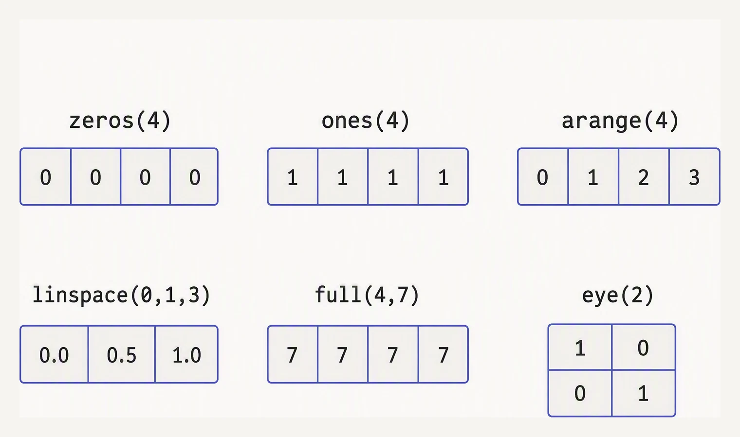
Pick by what you know: the values, the shape, or the range.
The simplest pattern: ask for a shape, and tell NumPy what to fill it with.
import numpy as np

# Placeholder for 128 embedding vectors of dim 768 (e.g., BERT outputs).
embeddings = np.zeros((128, 768), dtype=np.float32)
print("embeddings:", embeddings.shape, embeddings.dtype)

# Bias terms initialized to 1.0
bias = np.ones(768, dtype=np.float32)
print("bias      :", bias.shape, "sum =", bias.sum())

# A "mask" filled with a sentinel value (e.g., -1 for missing label).
labels = np.full((128,), fill_value=-1, dtype=np.int32)
print("labels    :", labels[:5], "...")
embeddings: (128, 768) float32
bias : (768,) sum = 768.0
labels : [-1 -1 -1 -1 -1] ...The pattern is always the same: pass the shape first, then an optional dtype. The default
dtype is float64, which is almost never what you want for big data — so be explicit.
import numpy as np

# DON'T do this:
buf = np.empty((3, 4))
print("uninitialized 'empty':")
print(buf)   # could be anything — old memory contents.

# DO this when you'll fill it immediately:
result = np.empty((1000,), dtype=np.float64)
for i in range(1000):
    result[i] = i ** 0.5   # we overwrite every slot before reading
print("first 5 filled:", result[:5])
uninitialized 'empty':
[[0. 0. 0. 0.]
[0. 0. 0. 0.]
[0. 0. 0. 0.]]
first 5 filled: [0. 1. 1.41421356 1.73205081 2. ]On this particular run the uninitialized buffer happened to come back all zeros — freshly-allocated
memory often does, which is exactly what makes empty so treacherous. It is luck, not a guarantee:
reuse a buffer later in a program and np.empty will hand you stale leftover values instead. The
DO half is the safe pattern — every slot is written (i ** 0.5) before anything reads it, so the
result is the clean [0, 1, √2, √3, 2, …].
Ranges — arange vs linspace
These two cover almost every “give me a sequence” need.
np.arange(start, stop, step)— like Python’srange, exclusive upper bound, you choose the step.np.linspace(start, stop, num)— inclusive on both ends, you choose the count.
import numpy as np

# arange: step = 0.5, stop is exclusive.
print("arange  :", np.arange(0, 3, 0.5))      # [0., 0.5, 1., 1.5, 2., 2.5]

# linspace: 7 points from 0 to 2π — exactly what you want for plotting sin(x).
x = np.linspace(0, 2 * np.pi, 7)
print("linspace:", x.round(3))

# Why linspace beats arange for floats: arange can miss the endpoint
# due to floating-point rounding.
print("arange to 1.0:", np.arange(0, 1.0, 0.1))       # 10 points, no 1.0
print("linspace 11  :", np.linspace(0, 1.0, 11))       # 11 points, includes 1.0
arange : [0. 0.5 1. 1.5 2. 2.5]
linspace: [0. 1.047 2.094 3.142 4.189 5.236 6.283]
arange to 1.0: [0. 0.1 0.2 0.3 0.4 0.5 0.6 0.7 0.8 0.9]
linspace 11 : [0. 0.1 0.2 0.3 0.4 0.5 0.6 0.7 0.8 0.9 1. ]Rule of thumb: integer step → arange. Float-spaced grid for plotting or numerical
integration → linspace. The reason arange drops the endpoint is the floating-point trap from
the numerical-stability lesson: it accumulates
start + k·step, and rounding can nudge the final value just past stop, so it is dropped.
linspace sidesteps this by computing each point independently as
start + k·(stop − start)/(num − 1) — which is why its endpoint is exact.
Identity and diagonals
import numpy as np

# Identity matrix — used in linear algebra and as a starting point for
# many transformations.
I = np.eye(4, dtype=np.float32)
print("eye(4):")
print(I)

# np.identity is the square-only variant — same result here.
print("identity(3):")
print(np.identity(3))
eye(4):
[[1. 0. 0. 0.]
[0. 1. 0. 0.]
[0. 0. 1. 0.]
[0. 0. 0. 1.]]
identity(3):
[[1. 0. 0.]
[0. 1. 0.]
[0. 0. 1.]]Random arrays — the modern API
The old np.random.rand(...) calls still work, but the modern way is to create a Generator
from np.random.default_rng(seed). It is faster, has more distributions, and — given a seed — is
perfectly reproducible.
import numpy as np

rng = np.random.default_rng(seed=2026)

# Uniform [0, 1) — good for stochastic masks, dropout.
u = rng.random((3, 4))
print("uniform:")
print(u.round(3))

# Gaussian (standard normal) — most common weight init.
w = rng.standard_normal((4, 4))
print("\nstandard normal:")
print(w.round(2))

# Integer labels — useful for fake datasets, batch sampling.
y = rng.integers(low=0, high=10, size=20)
print("\nintegers 0..9:", y)
uniform:
[[0.179 0.64 0.467 0.371]
[0.355 0.791 0.905 0.177]
[0.653 0.298 0.967 0.92 ]]
standard normal:
[[-0.06 -0.09 0.16 -0.61]
[-0.4 0.55 -0.13 -1.37]
[-0.48 0.66 -0.23 -0.15]
[ 0.64 1.82 -0.71 1.35]]
integers 0..9: [3 4 6 2 9 2 9 8 9 7 5 6 2 3 4 9 7 5 5 4]Because the seed is fixed at 2026, those exact numbers reproduce on any machine — and note
rng.integers(low=0, high=10, ...) returns values 0…9: the high bound is exclusive, so 10
never appears.
Decision tree
Quick reference for “which constructor do I want?”:
Need filler value 0?              → np.zeros(shape, dtype=...)
Need filler value 1?              → np.ones(shape, dtype=...)
Need a different filler?          → np.full(shape, value, dtype=...)
Need uninitialized (fast)?        → np.empty(shape)  — but fill it!
Need a stepped range?             → np.arange(start, stop, step)
Need N equally-spaced floats?     → np.linspace(start, stop, num)
Need an identity matrix?          → np.eye(n)
Need random values?               → rng = default_rng(); rng.random(shape)
In one breath
The shape-first constructors fill an array from a shape alone: zeros / ones /
full (value-filled), empty (uninitialized — fast but dangerous, only safe if you
overwrite every slot before reading), arange (you pick the step, upper bound exclusive,
can miss a float endpoint to rounding) vs linspace (you pick the count, both ends
inclusive, endpoint exact), eye/identity (identity matrix), and random via the modern
default_rng(seed) generator (.random, .standard_normal, .integers with an exclusive
high). The default dtype is float64 — almost never what you want at scale, so pass dtype=
explicitly.
Practice
Quick check
np.empty faster than np.zeros?np.random.rand(3,3) and np.random.default_rng().random((3,3))?A question to carry forward
Did you catch the refrain running through every constructor in this lesson? Pass the dtype. The
default float64 is almost never what you want. Be explicit. We kept issuing that warning and
never once justified it — what does the dtype actually buy you, what does it cost, and what breaks
if you ignore it?
The next lesson finally opens that box. What are the NumPy dtypes — how much memory and how
much numeric range each one gives you — and what are the silent, no-exception-raised overflow
and precision bugs they invite? The int8 that wraps around from 127 to −128 without a peep,
the float32 that quietly rounds your sum into noise: these are among the most baffling bugs in
all of numeric Python, precisely because nothing errors out.
Practice this in an interview
All questionsPython lists are heterogeneous, pointer-based, and general-purpose. NumPy arrays are homogeneous, stored as contiguous typed memory, and support vectorised operations that run at C speed. For numerical work on more than a few hundred elements, NumPy is almost always faster and more memory-efficient.
NumPy operations execute compiled C code over contiguous memory blocks in a single call, while a Python loop incurs interpreter overhead and dynamic type checks on every element. Vectorization means expressing an operation over an entire array at once so the hot path never re-enters the Python interpreter.
Vectorized pandas and NumPy operations operate on entire arrays in compiled C/Fortran code and should always be your first choice. apply runs a Python function row- or column-wise in a Python loop, map transforms a single Series element-by-element, and applymap (DataFrame.map in pandas 2.1+) applies a function to every scalar — all three are orders of magnitude slower than vectorized equivalents.
A list materialises all values in memory at once; a generator produces values one at a time on demand, using O(1) memory regardless of the sequence length. Prefer generators for large or infinite sequences, pipelines, and any situation where you do not need random access.