Einsum — one notation to rule them all
A single mental model — repeated indices sum, free indices stay — that expresses matmul, transpose, trace, and batched ops in one line.
Written and reviewed by Shreyash Prashu Last reviewed
What you'll learn
- The Einstein-summation rule that powers einsum
- How to translate matmul, transpose, and trace into einsum
- When einsum is the cleanest tool — and when it's a footgun
Before you start
The last lesson ended on a hunch: matmul, inner, outer, trace, transpose, batched matmul — a dozen
named operations that are secretly one move, multiply then sum over shared axes. np.einsum
(Einstein summation, the notation physicists use for tensor contractions) is that one move made
explicit.
The string 'bij,bjk->bik' looks intimidating the first time you meet it. But the rule underneath
is a single sentence — and once it clicks you can write almost any tensor operation in one line.
The one rule
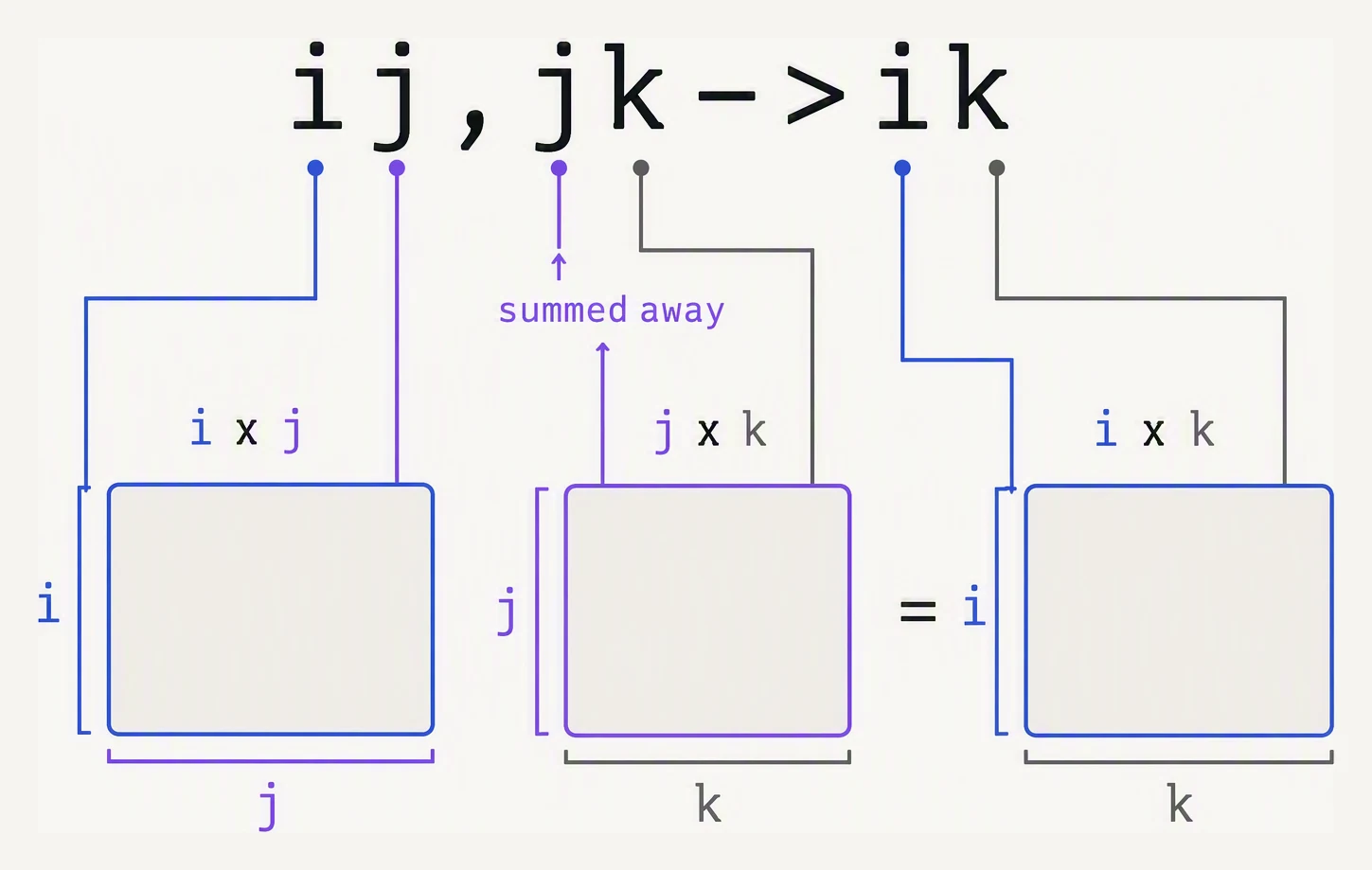
Repeated index means sum over it. Missing from the output means collapse it.
Indices that appear twice get summed. Indices that appear once stay.
That is the whole model. The string 'ij,jk->ik' reads as:
- inputs have shapes
(i, j)and(j, k) jappears in both inputs and not in the output → sum overjiandkappear once → keep them- so this is matrix multiplication
import numpy as np

rng = np.random.default_rng(0)
A = rng.standard_normal((3, 4))
B = rng.standard_normal((4, 5))

# These three lines compute the same thing
print(np.allclose(A @ B, np.einsum('ij,jk->ik', A, B)))
print(np.allclose(A @ B, np.matmul(A, B)))
True
True'ij,jk->ik' and A @ B are the same operation — einsum just spells out which axis (j) gets
contracted.
Hover an index to see it light up
The rule: repeated indices are summed (contracted); indices kept on the right survive (free).
ij,jk->ikCommon ops as einsum
The same rule covers a surprising amount of linear algebra — each op one or two characters from the next:
import numpy as np

rng = np.random.default_rng(0)
A = rng.standard_normal((4, 4))
v = rng.standard_normal(4)
M = rng.standard_normal((3, 5))

# Transpose: just reorder the output indices
print("transpose:", np.allclose(np.einsum('ij->ji', M), M.T))

# Trace: sum of the diagonal — the same index twice in input, none in output
print("trace:   ", np.allclose(np.einsum('ii->', A), np.trace(A)))

# Inner product u . v
u = rng.standard_normal(4)
print("inner:   ", np.allclose(np.einsum('i,i->', u, v), u @ v))

# Outer product u v^T  — no repeated index
print("outer:   ", np.allclose(np.einsum('i,j->ij', u, v), np.outer(u, v)))

# Diagonal — single repeated index, kept in output
print("diag:    ", np.allclose(np.einsum('ii->i', A), np.diag(A)))

# Sum all elements
print("sum all: ", np.allclose(np.einsum('ij->', M), M.sum()))
transpose: True
trace: True
inner: True
outer: True
diag: True
sum all: TrueSix different operations, one rule:
- Flip
'ij->ji'and you have a transpose. - Collapse both indices of a square matrix with
'ii->'and you have a trace. - Keep the repeated index with
'ii->i'and it is the diagonal instead.
That density is why research papers describe new architectures in einsum — it is more compact than prose and completely unambiguous.
Batched matmul — where einsum shines
Once you have a batch dimension, plain @ still works but reading the code gets harder. Einsum makes
the intent obvious:
import numpy as np

rng = np.random.default_rng(0)

# 32 samples in a batch, each a 64x128 matrix multiplied by a 128x16 matrix
A = rng.standard_normal((32, 64, 128))
B = rng.standard_normal((32, 128, 16))

# Three equivalent ways
C1 = A @ B
C2 = np.matmul(A, B)
C3 = np.einsum('bij,bjk->bik', A, B)

print("shapes:", C1.shape, C2.shape, C3.shape)
print("agree:", np.allclose(C1, C3))
shapes: (32, 64, 16) (32, 64, 16) (32, 64, 16)
agree: TrueThe b index says “this dimension is independent — repeat the operation along it.” In
'bij,bjk->bik' the j contracts (the matmul) while b just rides along untouched. That
convention scales: you can have several batch indices ('abij,abjk->abik') or different ones on
each side.
Attention — the canonical einsum example
A scaled-dot-product attention layer computes Q Kᵀ over a batch of heads. Without einsum it is a
tangle of transposes and reshapes; with einsum it is one line per operation:
import numpy as np

rng = np.random.default_rng(0)

# Standard transformer shapes
B, H, T, D = 2, 4, 16, 32   # batch, heads, tokens, head_dim
Q = rng.standard_normal((B, H, T, D))
K = rng.standard_normal((B, H, T, D))
V = rng.standard_normal((B, H, T, D))

# Scores = Q @ K^T  — one line, broadcast over (B, H)
scores = np.einsum('bhqd,bhkd->bhqk', Q, K) / np.sqrt(D)
print("scores shape:", scores.shape)   # (B, H, T, T) — token-to-token

# Softmax along the last axis, then mix V
def softmax(x):
    x = x - x.max(-1, keepdims=True)
    e = np.exp(x)
    return e / e.sum(-1, keepdims=True)

attn = softmax(scores)
out  = np.einsum('bhqk,bhkd->bhqd', attn, V)
print("out shape:   ", out.shape)
scores shape: (2, 4, 16, 16)
out shape: (2, 4, 16, 32)The two einsum strings read like the math. 'bhqd,bhkd->bhqk' sums over d (the head dimension)
to score every query against every key. It leaves (B, H, T, T), a token-to-token matrix per head.
'bhqk,bhkd->bhqd' then sums over k (the keys) to mix the values back to (B, H, T, D). No
transposes, no reshapes. Notice the stable softmax (subtract the max), straight from the
numerical-stability lesson.
When einsum is the wrong tool
Einsum is expressive, but it can be slower than the specialized op: np.matmul routes to BLAS
(your CPU’s hand-tuned linear-algebra library), and einsum’s contraction planner does not always
take that path.
The other risk is readability for teammates. If A @ B already says what you mean, prefer it. Save
einsum for the operations where the alternative is a gauntlet of transpose, reshape, and
swapaxes.
In one breath
np.einsum runs on one rule: repeated indices sum, free indices stay.
These translations cover six operations:
'ij,jk->ik'is matmul (contractj).'ij->ji'is transpose.'ii->'is trace.'ii->i'is diagonal.'i,j->ij'is outer.'ij->'is sum-all.
A batch index just rides along untouched ('bij,bjk->bik'). This makes batched/multi-head
operations readable.
Attention is two contractions:
'bhqd,bhkd->bhqk'produces scores and contractsd.'bhqk,bhkd->bhqd'mixes values and contractsk.
There are no transposes. Caveats:
- einsum can miss the BLAS fast path (
np.matmulis often faster — useoptimize=Trueand benchmark hot loops) - if
A @ Balready reads clearly, prefer it
Practice
Quick check
np.einsum('ij,j->i', A, x) compute when A is (m, n) and x is (n,)?'ii->' mean (note: empty output)?@ for batched matmul?A question to carry forward
Look back at almost every code block in this entire NumPy section. Each one opened with the same
incantation — rng = np.random.default_rng(seed) — conjuring reproducible random data we leaned on
for benchmarks, fake datasets, weight matrices, and these very attention inputs, yet never once
examined.
The final NumPy lesson pays that debt. It asks:
- What is a Generator?
- Why has
default_rngreplaced the oldnp.random.rand? - How does a single seed make “random” perfectly reproducible across machines and runs?
- Which distributions, shuffles, and choices power the simulations, train/test splits, weight initialisation, and dropout you will reach for every day?
Practice this in an interview
All questionsNumPy operations execute compiled C code over contiguous memory blocks in a single call, while a Python loop incurs interpreter overhead and dynamic type checks on every element. Vectorization means expressing an operation over an entire array at once so the hot path never re-enters the Python interpreter.
Vectorized pandas and NumPy operations operate on entire arrays in compiled C/Fortran code and should always be your first choice. apply runs a Python function row- or column-wise in a Python loop, map transforms a single Series element-by-element, and applymap (DataFrame.map in pandas 2.1+) applies a function to every scalar — all three are orders of magnitude slower than vectorized equivalents.
Python lists are heterogeneous, pointer-based, and general-purpose. NumPy arrays are homogeneous, stored as contiguous typed memory, and support vectorised operations that run at C speed. For numerical work on more than a few hundred elements, NumPy is almost always faster and more memory-efficient.
Sort the array, then fix one element at a time and run a two-pointer search on the remaining right portion to find pairs that sum to its negation. Careful duplicate-skipping at both the outer loop and the inner pointers is what makes the result unique. Overall complexity is O(n²).