Linear algebra with np.linalg
solve, inv, det, norm, eig, svd, qr, pinv — the linear algebra toolbox you need for regression, PCA, and recommender systems.
Written and reviewed by Shreyash Prashu Last reviewed
What you'll learn
- Why np.linalg.solve beats np.linalg.inv for solving Ax = b
- Eigendecomposition vs SVD — when each applies
- Pseudo-inverse for non-square systems
Before you start
The last lesson built linear transformations with @; this one runs them in reverse. np.linalg is
where NumPy keeps the heavy machinery — the routines that solve Ax = b, decompose a matrix
into its hidden axes, and back every regression, PCA, and recommender system. You don’t need to
re-derive the math (the math-for-ml chapter did that); you need to know which function to reach for,
and the one habit that separates working code from textbook code: never literally invert a
matrix.
solve > inv (almost always)
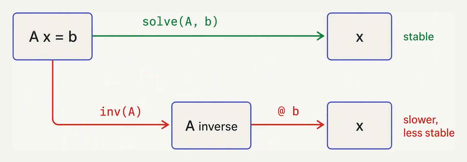
Never invert to solve. solve is faster and numerically safer.
The textbook writes x = A⁻¹ b to solve Ax = b. Don’t put that in code.
import numpy as np

# A small system: 3 equations, 3 unknowns
A = np.array([[3., 1., 2.],
              [1., 4., 1.],
              [2., 1., 5.]])
b = np.array([8., 10., 14.])

# The textbook way — slower and numerically worse
x_inv = np.linalg.inv(A) @ b

# The right way — faster, more accurate
x_solve = np.linalg.solve(A, b)

print("inv:   ", x_inv)
print("solve: ", x_solve)
print("residual (inv):   ", np.linalg.norm(A @ x_inv - b))
print("residual (solve): ", np.linalg.norm(A @ x_solve - b))   # tiny digits vary by CPU/BLAS
inv: [0.6 1.8 2.2]
solve: [0.6 1.8 2.2]
residual (inv): 0.0
residual (solve): 2.5121479338940403e-15solve uses an LU decomposition under the hood — roughly half the work of computing inv and
then multiplying. Here both land on the same answer [0.6, 1.8, 2.2] with residuals at the
floating-point floor (0 and ~2.5e-15 on our machine — the exact tiny digits vary by CPU), because this 3×3 is tiny and well-conditioned. The gap
opens up when A is large or ill-conditioned: inv’s extra round-trip through an explicit
inverse amplifies round-off, often by orders of magnitude, while solve stays tight. Same answer
here; very different behaviour at scale.
Linear regression via the normal equations
The “normal equations” give the least-squares fit β = (XᵀX)⁻¹ Xᵀy. We solve them properly —
without ever calling inv.
import numpy as np

rng = np.random.default_rng(0)

# Synthetic data: y = 2*x1 + 3*x2 + 1 + noise
n = 200
X = rng.standard_normal((n, 2))
y = 2 * X[:, 0] + 3 * X[:, 1] + 1 + rng.standard_normal(n) * 0.1

# Add an intercept column
X_design = np.column_stack([X, np.ones(n)])

# Normal equations: (X'X) beta = X'y
# Solve for beta without ever inverting
XtX = X_design.T @ X_design
Xty = X_design.T @ y
beta = np.linalg.solve(XtX, Xty)

print(f"beta1 = {beta[0]:.3f}  (true 2.000)")
print(f"beta2 = {beta[1]:.3f}  (true 3.000)")
print(f"intercept = {beta[2]:.3f}  (true 1.000)")
beta1 = 1.995 (true 2.000)
beta2 = 3.012 (true 3.000)
intercept = 1.000 (true 1.000)That is the entire fit — and it recovered the true slopes (2, 3) and intercept (1) to within the
noise. sklearn.linear_model.LinearRegression is doing essentially this, plus some checks and a
sturdier solver path.
Determinant and norm
det measures how much a matrix scales volumes — zero determinant means the matrix is singular
(no inverse). norm measures magnitude: for vectors the Euclidean length, for matrices the
Frobenius norm by default.
import numpy as np

A = np.array([[2., 1.],
              [1., 3.]])

print("det A =", np.linalg.det(A))         # nonzero → invertible
print("||A|| =", np.linalg.norm(A))         # Frobenius
print("||A||_2 =", np.linalg.norm(A, 2))    # spectral (largest singular value)

# Vector norm
v = np.array([3., 4.])
print("||v||  =", np.linalg.norm(v))        # 5.0
print("||v||_1 =", np.linalg.norm(v, 1))    # sum of |components|
det A = 5.000000000000001
||A|| = 3.872983346207417
||A||_2 = 3.6180339887498953
||v|| = 5.0
||v||_1 = 7.0det A = 5 (nonzero, so invertible); the classic 3-4-5 triangle gives ||v|| = 5.0 while the L1
norm sums to 7.0. (The trailing …001 on the determinant is floating point’s “5” — the
numerical-stability lesson again.)
Eigendecomposition
An eigenvalue λ and its eigenvector v satisfy A @ v = λ·v: the matrix only scales
v, never rotates it. eig returns all such pairs. For a symmetric / Hermitian matrix use
eigh — it exploits the symmetry for speed and is guaranteed to return real (not complex) values:
import numpy as np

# A symmetric matrix (e.g. a covariance matrix)
A = np.array([[4., 1., 0.],
              [1., 3., 1.],
              [0., 1., 2.]])

vals, vecs = np.linalg.eigh(A)
print("eigenvalues:", vals)
print("eigenvectors (columns):\n", vecs)

# Sanity check: A @ v == lambda * v
v0 = vecs[:, 0]
print("A @ v0:   ", A @ v0)
print("lam0 * v0:", vals[0] * v0)
eigenvalues: [1.26794919 3. 4.73205081]
eigenvectors (columns):
[[ 0.21132487 0.57735027 -0.78867513]
[-0.57735027 -0.57735027 -0.57735027]
[ 0.78867513 -0.57735027 -0.21132487]]
A @ v0: [ 0.26794919 -0.73205081 1. ]
lam0 * v0: [ 0.26794919 -0.73205081 1. ]The sanity check is the whole definition made concrete: A @ v0 and λ₀ · v0 print the same
vector, so multiplying by A did nothing but stretch v0 by λ₀ ≈ 1.268. Eigendecomposition only
works on square matrices; for everything else you reach for SVD.
SVD — the workhorse
SVD factors any matrix as A = U Σ Vᵀ. It powers PCA, recommender systems, image compression,
and least-squares solvers. If you learn one decomposition, learn this one.
import numpy as np

rng = np.random.default_rng(7)

# A rank-deficient matrix — singular values reveal the rank
A = rng.standard_normal((5, 3)) @ rng.standard_normal((3, 8))
print("A shape:", A.shape)

U, s, Vt = np.linalg.svd(A, full_matrices=False)
print("U:", U.shape, "s:", s.shape, "Vt:", Vt.shape)
print("singular values:", s.round(3))
A shape: (5, 8)
U: (5, 5) s: (5,) Vt: (5, 8)
singular values: [6.29 3.527 1.4 0. 0. ]Five singular values, but only three are nonzero — exactly the rank of a (5,3) @ (3,8)
product, which can be at most 3. The two zeros are the SVD announcing “there is no real structure
here.” Keep the top k and you get a low-rank approximation:
import numpy as np

rng = np.random.default_rng(7)
A = rng.standard_normal((5, 3)) @ rng.standard_normal((3, 8))

U, s, Vt = np.linalg.svd(A, full_matrices=False)

# Rank-2 approximation
k = 2
A_approx = U[:, :k] @ np.diag(s[:k]) @ Vt[:k, :]
print("error (Frobenius):", round(np.linalg.norm(A - A_approx), 10))
# By the Eckart-Young theorem, this equals sqrt(sum of s[k:]**2)
print("sqrt(sum of dropped s²):", round(np.sqrt(np.sum(s[k:]**2)), 10))
error (Frobenius): 1.3995981525
sqrt(sum of dropped s²): 1.3995981525The two numbers match to the last digit — that is the Eckart–Young theorem: the error of the
best rank-k approximation is exactly the norm of the singular values you dropped. This is
truncated SVD, the technique behind Netflix-era recommenders: factor the (user × movie) matrix,
keep the top k components.
QR and pinv
qr factors A = QR with Q orthogonal and R upper-triangular — least squares with good stability
and less cost than SVD. pinv is the Moore–Penrose pseudo-inverse, the right tool for
non-square or singular matrices where inv would simply fail:
import numpy as np

# A non-square matrix — np.linalg.inv would fail
A = np.array([[1., 2.],
              [3., 4.],
              [5., 6.]])

A_pinv = np.linalg.pinv(A)
print("pinv shape:", A_pinv.shape)         # (2, 3)
print("A_pinv @ A =\n", (A_pinv @ A).round(6) + 0.0)   # ≈ identity (+ 0.0 tidies -0.)
pinv shape: (2, 3)
A_pinv @ A =
[[1. 0.]
[0. 1.]]The (3, 2) matrix has no true inverse, but its (2, 3) pseudo-inverse satisfies A⁺A = I — a
left inverse. For least squares specifically, np.linalg.lstsq(A, b) wraps this up with extra
diagnostics; prefer it when you are actually solving Ax ≈ b in the over- or under-determined case.
In one breath
np.linalg is the heavy linear-algebra toolbox. Always solve(A, b), never inv(A) @ b —
LU-based, ~half the work and far stabler when A is ill-conditioned (the regression demo fits the
normal equations this way, recovering slopes 2, 3 and intercept 1). det flags singularity
(zero = no inverse), norm measures magnitude (Frobenius for matrices, Euclidean/L1/L2 for
vectors). eig/eigh give eigenpairs A v = λ v (use eigh for symmetric matrices → real
values); svd factors any matrix A = UΣVᵀ, its singular values exposing the rank (three
nonzero here), and a truncated top-k SVD is the optimal low-rank approximation (Eckart–Young).
For non-square/singular systems, pinv / lstsq.
Practice
Quick check
Ax = b. Which is best?A question to carry forward
Notice how many named operations have piled up across this chapter and the last — @, np.dot,
inner, outer, trace, transpose, solve, batched matmul. They feel like a dozen separate
tools, but squint and they are all the same primitive move: multiply elements, then sum over the
axes the two operands share. Matmul sums over the inner axis; trace sums over a repeated axis; an
outer product sums over nothing at all.
Is there a single notation that captures every one of them — and lets you write a batched,
multi-head attention score in one readable line instead of a thicket of transposes and reshapes?
There is, and physicists have used it for a century. The next lesson is np.einsum: one rule —
repeated indices sum, free indices stay — that spells matmul, transpose, trace, and batched
contraction all in the same breath.
Practice this in an interview
All questionsPCA centers data and finds orthogonal directions that maximize variance, usually through the covariance matrix's eigenvectors or an SVD, then projects observations onto the leading directions. Choose the component count using cumulative explained variance or reconstruction needs for compression, and cross-validated downstream performance for prediction; standardize first only when feature scales should contribute equally.
Under full column rank, OLS sets the gradient of the squared-error objective to zero, giving the normal equations and the unique coefficient vector β = (XᵀX)⁻¹Xᵀy. In rank-deficient or numerical settings, use the pseudoinverse or a least-squares solver rather than explicitly forming the inverse.
PCA finds the orthogonal directions of maximum variance in the data and projects onto a lower-dimensional subspace, reducing features while retaining most information. It is most useful before distance-based models or when training is bottlenecked by dimensionality. Its main limits are loss of interpretability, sensitivity to scale, and an assumption of linear structure.
ElasticNet addresses the tension between Lasso's sparse but potentially unstable feature selection and Ridge's stable but dense treatment of correlated predictors. Its L1 and L2 penalties can share signal across correlated features while still setting some coefficients exactly to zero, although it does not guarantee that every correlated group will be selected together.