Reshape and axes
reshape, transpose, swapaxes, newaxis, squeeze — moving data between shapes without copying.
Written and reviewed by Shreyash Prashu Last reviewed
What you'll learn
-
reshapevsravelvsflatten— when each returns a view - Transposing and swapping axes for tensor layouts
-
expand_dims,squeeze, andnp.newaxisfor broadcasting - The
-1shortcut for inferring a dimension
Before you start
The last lesson promised a payoff, and here it is. Indexing lifted pieces out of an array; reshaping changes the array’s shape while leaving every value exactly where it sits.
The reason it is almost always free is the strides idea from a few lessons back. The data is
one flat block, the shape is merely a recipe for reading it, and reshape rewrites the recipe without
moving a single byte. That matters because data rarely arrives in the shape your model wants. You
load images as (H, W, C) and the framework wants (C, H, W); you get a flat feature vector and
need a batch of rows. Reshape bridges the gap at zero copy cost.
reshape — change the shape, keep the data
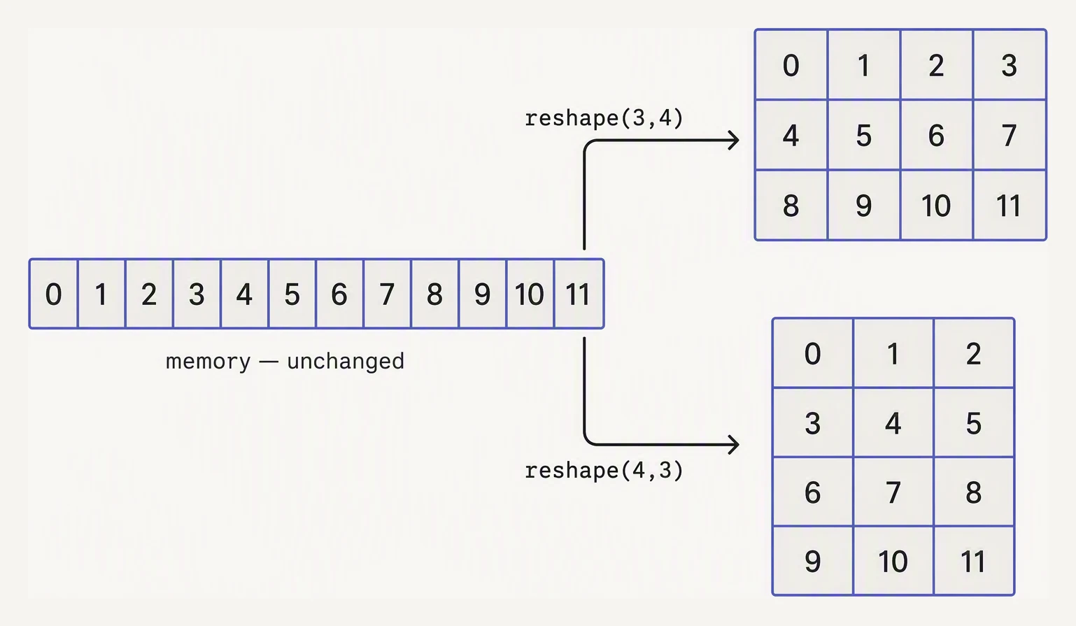
Reshape never moves data — it only changes how the same run of memory is read.
arr.reshape(new_shape) returns a view with the same data, read under a new shape — no copy,
the same memory just interpreted differently. The total number of elements must stay the same.
Note:
reshapereturns a view when the memory layout allows it (contiguous arrays usually qualify). If not — e.g. after a non-trivial transpose — NumPy falls back to a copy. Checkarr.base is not Noneto confirm you have a view.
import numpy as np

# 24 pixel values — flatten of an image we haven't unfolded yet.
flat = np.arange(24)
print("flat shape:", flat.shape)

# Unfold to 4×6.
mat = flat.reshape(4, 6)
print("\nreshape(4, 6):")
print(mat)

# Or 2×3×4 (a "color image" of 2 rows, 3 cols, 4 channels).
cube = flat.reshape(2, 3, 4)
print("\nreshape(2, 3, 4) — first slice:")
print(cube[0])
flat shape: (24,)
reshape(4, 6):
[[ 0 1 2 3 4 5]
[ 6 7 8 9 10 11]
[12 13 14 15 16 17]
[18 19 20 21 22 23]]
reshape(2, 3, 4) — first slice:
[[ 0 1 2 3]
[ 4 5 6 7]
[ 8 9 10 11]]The same 0–23 run of numbers was read as a 4×6 grid and then a 2×3×4 cube — same bytes, two
shapes. The -1 shortcut lets NumPy infer one dimension from the rest. It is the workhorse for
“I don’t care exactly how many rows, just give me 3 columns”:
import numpy as np

x = np.arange(60)

# "Give me 3 columns, figure out the rows."
print(x.reshape(-1, 3).shape)     # (20, 3)

# "Give me 5 rows, figure out the columns."
print(x.reshape(5, -1).shape)     # (5, 12)

# Flatten by inferring a single axis.
print(x.reshape(-1).shape)        # (60,)
(20, 3)
(5, 12)
(60,)You can use -1 exactly once per call, and NumPy errors if the inferred dimension would not be a
whole number.
Pour the same 12 elements into a new shape
Below is a flat buffer — np.arange(12). Pick a target shape and watch the elements flow into it. Nothing moves in memory; reshape just reinterprets this one buffer under a new shape, filling in C order (row-major) by default. Try F order to fill column-major instead.
arr.reshape(3, 4) → (3, 4)view · no copyThe aha: reshape never moves data — it reinterprets the same flat buffer under a new shape, and (when the layout allows) returns a view, not a copy. -1 means “infer this dim from the rest.”
ravel vs flatten — view vs copy
Both turn an N-D array into a 1-D one. The difference is what they return:
ravel()— returns a view when possible (so cheap, but mutations propagate).flatten()— always returns a copy (safe to mutate).
import numpy as np

A = np.arange(12).reshape(3, 4)

r = A.ravel()
f = A.flatten()

r[0] = 999       # might affect A…
print("A after r[0]=999:")
print(A)

f[0] = -1        # …never affects A
print("\nf after f[0]=-1:", f[:5])
print("A unchanged:")
print(A)
A after r[0]=999:
[[999 1 2 3]
[ 4 5 6 7]
[ 8 9 10 11]]
f after f[0]=-1: [-1 1 2 3 4]
A unchanged:
[[999 1 2 3]
[ 4 5 6 7]
[ 8 9 10 11]]r[0] = 999 reached straight into A (ravel gave a view). f[0] = -1 left A untouched (flatten
copied). For read-only use prefer ravel (free); when you need a buffer you can safely mutate,
use flatten (or ravel().copy()).
Transpose — swap axes
arr.T swaps all axes. For 2-D, that is the familiar matrix transpose; for higher-D, the axes
reverse.
import numpy as np

A = np.arange(12).reshape(3, 4)
print("A:")
print(A)
print("A.T:")
print(A.T)

# For tensors with > 2 axes, use transpose(order) to specify the new axis order.
img = np.zeros((480, 640, 3), dtype=np.uint8)   # H, W, C
img_chw = img.transpose(2, 0, 1)                # C, H, W
print("\nimage HWC :", img.shape)
print("image CHW :", img_chw.shape)
A:
[[ 0 1 2 3]
[ 4 5 6 7]
[ 8 9 10 11]]
A.T:
[[ 0 4 8]
[ 1 5 9]
[ 2 6 10]
[ 3 7 11]]
image HWC : (480, 640, 3)
image CHW : (3, 480, 640)transpose((2, 0, 1)) reads as: “old axis 2 becomes new axis 0, old axis 0 becomes new axis 1,
old axis 1 becomes new axis 2.” It is just a permutation of the axis order.
newaxis, expand_dims, squeeze
To make a 1-D array line up as a row or column — so it will broadcast against a matrix (next lesson) — you add an axis of length 1. There are three equivalent ways:
import numpy as np

v = np.array([1.0, 2.0, 3.0, 4.0])    # shape (4,)
print("v.shape:", v.shape)

# As a column vector (4, 1)
col1 = v[:, np.newaxis]
col2 = v[:, None]                     # None is an alias for np.newaxis
col3 = np.expand_dims(v, axis=1)
print("column shape:", col1.shape, col2.shape, col3.shape)

# As a row vector (1, 4)
row = v[np.newaxis, :]
print("row shape   :", row.shape)
v.shape: (4,)
column shape: (4, 1) (4, 1) (4, 1)
row shape : (1, 4)The reverse — removing axes of length 1 — is squeeze:
import numpy as np

# A model output of shape (1, 1, 10) — a single batch, single channel, 10 logits.
logits = np.zeros((1, 1, 10))
print("before squeeze:", logits.shape)

print("squeeze all   :", np.squeeze(logits).shape)         # (10,)
print("squeeze axis=0:", np.squeeze(logits, axis=0).shape) # (1, 10)
before squeeze: (1, 1, 10)
squeeze all : (10,)
squeeze axis=0: (1, 10)You will reach for squeeze constantly when pulling a prediction out of a model that returns
batched outputs but you fed it just one example.
A real-world reshape — image batches
The canonical DataLoader pattern: turn a list of images into one batch tensor in the framework’s expected layout.
import numpy as np

# Simulate 8 random 32×32 RGB images, loaded as HWC uint8.
rng = np.random.default_rng(0)
images = [rng.integers(0, 256, size=(32, 32, 3), dtype=np.uint8)
          for _ in range(8)]
print("one image    :", images[0].shape)

# Stack into a batch: (N, H, W, C).
batch_hwc = np.stack(images, axis=0)
print("batch HWC    :", batch_hwc.shape)

# Convert to channels-first for PyTorch: (N, C, H, W).
batch_chw = batch_hwc.transpose(0, 3, 1, 2)
print("batch CHW    :", batch_chw.shape)

# Cast to float32 and normalize to [0, 1].
batch_f32 = batch_chw.astype(np.float32) / 255.0
print("batch f32    :", batch_f32.shape, batch_f32.dtype,
      "min:", batch_f32.min(), "max:", batch_f32.max())
one image : (32, 32, 3)
batch HWC : (8, 32, 32, 3)
batch CHW : (8, 3, 32, 32)
batch f32 : (8, 3, 32, 32) float32 min: 0.0 max: 1.0That four-line pipeline — stack → transpose → astype → divide — is the backbone of nearly every
image data loader written in the last decade.
In one breath
- Reshape rewrites the shape recipe over the same flat data, so it is free (a view) when the
layout allows —
reshape(4, 6)andreshape(2, 3, 4)re-read one 0–23 run, and-1infers one axis (reshape(-1, 3)→(20, 3)). ravelflattens to a view when possible, whileflattenalways copies (mutating the ravel hitA, the flatten didn’t).- Transpose permutes axes —
arr.Treverses all of them, andtranspose(2, 0, 1)turns HWC into CHW for PyTorch. - Add a length-1 axis with
np.newaxis/None/expand_dims(to set up broadcasting) and drop length-1 axes withsqueeze. - The everyday image-loader pipeline is just
stack → transpose → astype → /255.
Practice
Quick check
img with shape (224, 224, 3). You want a (3, 224, 224) array for PyTorch. Which does it?arr.ravel() and arr.flatten()?x with shape (50,) and want to add it as a column to a (50, 10) matrix. What's the right reshape?A question to carry forward
Notice how many times this lesson reached for one move — v[:, np.newaxis], expand_dims, a
(50, 1) column — and justified it with the same unexplained word: “so it will broadcast.” We
kept reshaping arrays into length-1 axes specifically to line them up against bigger ones, on
faith that NumPy would then “stretch” the small one to fit.
That stretching has a name and a precise rule, and it is the engine that makes vectorised code
actually work. What is broadcasting — how does NumPy combine a (3,) vector with every row
of a (4, 3) matrix, or a column with a row to fill an entire grid, without a single loop? What
exactly decides when two shapes click together versus throw “could not broadcast”?
Practice this in an interview
All questionspivot reshapes long-format data to wide by spreading a column's values into new column headers — it requires unique index/column combinations and has no aggregation. pivottable is the aggregating version that handles duplicates via a specified aggfunc. melt is the inverse: it takes wide-format data and collapses multiple columns into key-value rows (long format).
Wide format stores multiple measurements as separate columns per subject; long (tidy) format stores one measurement per row with a variable-name column and a value column. Long format is required by most statistical and visualization libraries, makes adding new variables trivial, and is the standard expected by groupby and merge operations.
concat stacks DataFrames along an axis without matching keys; join aligns on the index (or a single key column) using a convenient shorthand; merge is the most general, joining on any column(s) with full SQL-style control over the join type, key names, and suffix handling.
Vectorized pandas and NumPy operations operate on entire arrays in compiled C/Fortran code and should always be your first choice. apply runs a Python function row- or column-wise in a Python loop, map transforms a single Series element-by-element, and applymap (DataFrame.map in pandas 2.1+) applies a function to every scalar — all three are orders of magnitude slower than vectorized equivalents.