The five distributions you'll actually use
Bernoulli, Binomial, Uniform, Normal, Exponential. Each one models a different real-world situation. Sample from them, plot them, recognize them in the wild.
Written and reviewed by Shreyash Prashu Last reviewed
What you'll learn
- The shapes and use-cases of the five distributions worth memorizing
- The difference between PMF (discrete) and PDF (continuous)
- How to sample any of them with
np.random - Why the normal distribution shows up so often (preview of CLT)
Before you start
Bayes left us a clue: a prior is not a number but a shape — the coin demo’s belief was a whole curve. Probabilities live as distributions, so it pays to know the common ones on sight. There are dozens of named distributions; you will meet exactly five over and over in ML and data science:
Bernoulli    — single yes/no   (one click, one click-no)
Binomial     — sum of N Bernoullis (clicks in 1000 impressions)
Uniform      — equally likely    (a random pick from [a, b])
Normal       — bell curve        (most measurement errors, sample means)
Exponential  — waiting time      (time between events)
Learn the shape, the formula for sampling, and one situation where each shows up. That’s enough to read 90% of papers and dashboards.
Discrete vs continuous — PMF vs PDF
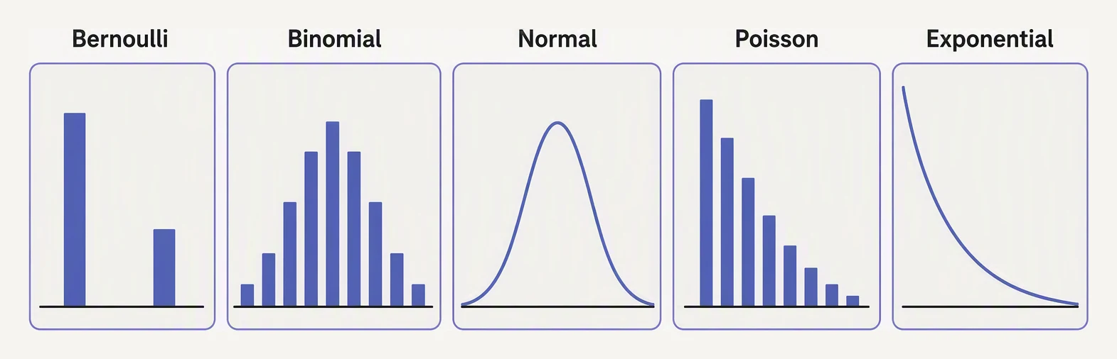
Five shapes worth recognising on sight.
Discrete distributions assign probability to specific outcomes. The list of those probabilities is called the probability mass function (PMF):
P(X = k) = some number with Σ_k P(X = k) = 1Continuous distributions can’t put non-zero probability on any single point — if they did, the infinite sum over all points would exceed 1. Instead they have a probability density function (PDF) — a curve whose area between two values gives the probability of landing in that range.
P(a ≤ X ≤ b) = ∫_a^b pdf(x) dx with ∫ pdf(x) dx = 1A common beginner trap: PDF values aren’t probabilities and can be greater than 1. They’re densities. Probability is what you get when you integrate (sum) them over an interval.
Drag the handles to read off a probability
Bernoulli — a single yes/no
One trial with probability p of success.
P(X = 1) = p,  P(X = 0) = 1 - p
E[X] = p
This is the smallest non-trivial distribution. “Did the user click?” “Did the email get opened?” “Is this loan in default?” — all Bernoulli.
import numpy as np

rng = np.random.default_rng(0)

p = 0.3
samples = rng.binomial(n=1, p=p, size=10_000)   # 0/1 outcomes
print("First 20 samples:", samples[:20])
print("Empirical p:", samples.mean(), "vs true:", p)
First 20 samples: [0 0 0 0 1 1 0 1 0 1 1 0 1 0 1 0 1 0 0 0]
Empirical p: 0.3001 vs true: 0.3Ten thousand 0/1 draws average to 0.3001 — the empirical p landing right on the true 0.3, as it must.
Binomial — sum of N Bernoullis
N independent Bernoulli trials, all with the same p. The binomial
counts how many were successes:
P(X = k) = C(N, k) · p^k · (1-p)^(N-k)
E[X] = N · p
“Out of 1000 ad impressions with click rate 5%, how many clicks do we expect?” Binomial.
import numpy as np
import matplotlib.pyplot as plt

rng = np.random.default_rng(0)

N, p = 1000, 0.05
samples = rng.binomial(n=N, p=p, size=10_000)   # 10,000 experiments
print(f"Mean # clicks per 1000 impressions: {samples.mean():.2f}  (expected {N*p})")
print(f"Std dev:                            {samples.std():.2f}")

fig, ax = plt.subplots(figsize=(6, 3.5))
ax.hist(samples, bins=30, color="steelblue", alpha=0.8)
ax.set_xlabel("Clicks per 1000 impressions")
ax.set_ylabel("Frequency")
ax.set_title(f"Binomial(N=1000, p=0.05): 10,000 simulated experiments")
plt.tight_layout()
plt.show()
Mean # clicks per 1000 impressions: 49.88 (expected 50.0)
Std dev: 6.94The mean clicks land at 49.88, right on the expected N·p = 50, with a spread of about 7. The histogram (plt.show()) already looks like a bell — that’s the central limit theorem sneaking in. With small N it looks chunkier and skewed; with big N it converges to a normal.
Uniform — everything equal
Every value in [a, b] is equally likely. The PDF is a constant
1/(b-a) between the bounds, zero outside.
E[X] = (a + b) / 2In ML you mostly use uniform for initialization (uniform random weights) and sampling within a fixed range (hyperparameter search, shuffling indices).
import numpy as np

rng = np.random.default_rng(0)

# Uniform between 0 and 10
samples = rng.uniform(0, 10, size=10_000)
print(f"Mean: {samples.mean():.4f}  Min: {samples.min():.4f}  Max: {samples.max():.4f}")

# Discrete uniform -- pick an integer in [low, high)
indices = rng.integers(0, 100, size=5)
print("Random indices:", indices)
Mean: 4.9941 Min: 0.0011 Max: 10.0000
Random indices: [21 56 48 96 42]The mean sits at 4.99 — dead centre of [0, 10], exactly (a+b)/2 — and the min and max hug the bounds, since every value in the range is equally likely.
Normal — the bell curve
The normal (or Gaussian) distribution is parameterized by mean μ
and standard deviation σ:
PDF(x) = (1 / (σ√(2π))) · exp(-(x - μ)² / (2σ²))You don’t memorize that formula — you memorize the shape: symmetric, bell-shaped, ~68% within 1σ of the mean, ~95% within 2σ.
It’s everywhere because of the central limit theorem (next lesson): averages of many independent things become approximately normal, regardless of the underlying distribution.
import numpy as np
import matplotlib.pyplot as plt

from scipy.stats import norm

rng = np.random.default_rng(0)

# Two normals
samples = rng.normal(loc=0, scale=1, size=10_000)
print(f"Mean: {samples.mean():.3f}  Std: {samples.std():.3f}  (target 0, 1)")

x = np.linspace(-5, 5, 200)
fig, ax = plt.subplots(figsize=(6, 3.5))
ax.hist(samples, bins=40, density=True, alpha=0.6, label="samples")
ax.plot(x, norm.pdf(x, 0, 1), lw=2, label="N(0,1) PDF")
ax.plot(x, norm.pdf(x, 1, 0.5), lw=2, label="N(1, 0.5) PDF")
ax.set_xlabel("x"); ax.set_ylabel("density")
ax.set_title("Normal distribution PDF (and 10k samples)")
ax.legend()
plt.tight_layout()
plt.show()
Mean: 0.006 Std: 0.998 (target 0, 1)The 10,000 samples average 0.006 with a standard deviation of 0.998 — a near-perfect N(0, 1). The plot (plt.show()) lays the sample histogram under the smooth N(0,1) curve (they match) and adds a taller, narrower N(1, 0.5) — narrower because a smaller σ concentrates the density and pushes its peak above 1, a reminder that PDF values are not probabilities.
Exponential — waiting times
The exponential distribution models the waiting time between events that happen randomly at a constant average rate. Inter-arrival times of customers, time until a server fails, time to next click.
PDF(x) = λ exp(-λ x)   for x ≥ 0
E[X] = 1 / λ
“Rate” λ is “events per unit time.” Mean wait is 1/λ (a rate of 2
per second → average wait of 0.5 second).
import numpy as np
import matplotlib.pyplot as plt

rng = np.random.default_rng(0)

# Mean wait = 5 seconds, so rate λ = 1/5
samples = rng.exponential(scale=5.0, size=10_000)
print(f"Mean: {samples.mean():.2f}  (expected 5.0)")

x = np.linspace(0, 25, 200)
lam = 1 / 5.0
pdf = lam * np.exp(-lam * x)

fig, ax = plt.subplots(figsize=(6, 3.5))
ax.hist(samples, bins=40, density=True, alpha=0.6, label="samples")
ax.plot(x, pdf, lw=2, label="Exp(λ=1/5) PDF")
ax.set_xlabel("Wait time"); ax.set_ylabel("density")
ax.set_title("Exponential distribution")
ax.legend()
plt.tight_layout()
plt.show()
Mean: 4.96 (expected 5.0)The average wait lands at 4.96 against the expected 1/λ = 5.0. The plot (plt.show()) shows the tell-tale shape — a tall spike near zero decaying to a long right tail: most waits are short, but the occasional long one does happen. Exponential is skewed right, never negative.
Putting it together — a simulated A/B test
You can recognize each piece. A user converts: Bernoulli. Conversions
across n users: Binomial. The difference between two groups’ rates,
divided by its standard error: approximately Normal (CLT). That’s the
machinery of an A/B test, two lessons from now.
import numpy as np

rng = np.random.default_rng(7)

# Two groups, A and B, each with n users
n = 5000
p_A = 0.050   # 5.0% conversion
p_B = 0.058   # 5.8% conversion

conversions_A = rng.binomial(n=n, p=p_A, size=1)[0]
conversions_B = rng.binomial(n=n, p=p_B, size=1)[0]

print(f"Group A: {conversions_A}/{n}  = {conversions_A/n:.4f}")
print(f"Group B: {conversions_B}/{n}  = {conversions_B/n:.4f}")
print(f"Observed lift: {(conversions_B - conversions_A) / n:.4f}")
Group A: 252/5000 = 0.0504
Group B: 286/5000 = 0.0572
Observed lift: 0.0068Each group is a single Binomial draw — 252 and 286 conversions — landing near their true 5.0% and 5.8% rates, for an observed lift of 0.68%. Whether a lift that size is real or just two Binomials wobbling is the question the A/B-test lesson answers; the distributions here are the raw material.
In one breath
Five distributions cover most of ML: Bernoulli (one yes/no, mean p), Binomial (count of N Bernoullis, mean Np), Uniform (all values in [a, b] equally likely — initialization and search), Normal (the bell, symmetric around μ, ~68% / 95% within 1σ / 2σ — everywhere, because of the CLT), and Exponential (right-skewed waiting times between random events, mean 1/λ). Discrete ones have a PMF — probability on each outcome, summing to 1; continuous ones have a PDF — a density whose area over an interval is the probability, so a density value can exceed 1 and P(X = exact point) = 0. Any of them samples in one line of np.random, which is why simulation can answer questions the algebra cannot.
Practice
Quick check
A question to carry forward
Every sample here came for free: rng.normal, rng.binomial, rng.exponential — one line each, because NumPy already knows the recipe for these famous shapes. But that is exactly the catch. The most useful distribution in Bayesian work is the posterior you just learned to build — prior times likelihood — and it almost never has a name or a built-in sampler. You can write down its formula, yet there is no rng.my_weird_posterior() to draw from it.
So here is the thread onward: given an arbitrary distribution you can evaluate but not directly draw from, how do you generate samples anyway? How does pushing a uniform random number through the inverse CDF conjure samples of any shape; when does rejection sampling let you sample by throwing darts; and what is MCMC — the method that made modern Bayesian inference possible by sampling distributions no one can write a formula to invert?
Practice this in an interview
All questionsA Bernoulli(p) trial is the atomic unit: a single experiment with success probability p. Binomial(n, p) is the sum of n independent, identically distributed Bernoulli(p) trials, counting total successes. Because Binomial is a sum of independent random variables, its mean and variance are n times those of a single Bernoulli.
The chi-square test assesses whether observed categorical frequencies differ from expected frequencies (goodness-of-fit) or whether two categorical variables are independent of each other (test of independence). It requires count data, a sufficiently large sample, and expected cell counts of at least 5.
Each distribution has a natural generative story: Bernoulli is a single coin flip; Binomial sums Bernoullis; Poisson counts rare arrivals; Normal emerges from sums of many small effects; Exponential models waiting times between Poisson events; Uniform assigns equal probability across a range. Choosing correctly comes from matching that story to the data-generating process.
An Exponential random variable satisfies P(X > s+t | X > s) = P(X > t): the remaining waiting time has the same distribution regardless of how long you have already waited. This is the only continuous distribution with this property, and it directly corresponds to a constant hazard rate — neither ageing nor improving over time.
A long-tailed distribution has tail probabilities that decay much more slowly than the exponential — meaning extreme events are far more common than a Gaussian model would predict. They appear in internet traffic, wealth, natural language word frequency, and insurance claims, and they invalidate many standard statistical techniques that assume thin tails.
Mean is optimal for symmetric, outlier-free data; median is the go-to for skewed distributions or when outliers are real rather than errors; mode is the only sensible average for nominal/categorical data. Robustness is a formal concept — the median's breakdown point is 50%, meaning half the data can be corrupted before it fails, while the mean's breakdown point is essentially 0%.
The normal distribution is a symmetric, bell-shaped probability distribution completely described by its mean and standard deviation. The empirical rule states that approximately 68%, 95%, and 99.7% of observations fall within one, two, and three standard deviations of the mean respectively — a direct consequence of integrating the Gaussian density over those intervals.
Parametric tests assume the data follow a specific distribution (usually normal) and make inferences about distributional parameters like the mean. Non-parametric tests make no such distributional assumption and typically operate on ranks. Non-parametric tests are more robust but less powerful when parametric assumptions genuinely hold.
Skewness measures the asymmetry of a distribution's tails — positive skew means a longer right tail, negative skew a longer left tail. Kurtosis measures the heaviness of the tails relative to a normal distribution; excess kurtosis above zero indicates more probability mass in the tails and peak than a Gaussian, which matters for risk and outlier frequency.
Use a z-test when the population standard deviation is known and the sample is large (n >= 30, by convention); use a t-test when the standard deviation must be estimated from the sample, which is almost always the case in practice. For large n the two tests converge, but the t-test is the safe default.
Variance is the average squared deviation from the mean; standard deviation is its square root and lives in the same units as the data. Variance is mathematically tractable — variances of independent variables add — while standard deviation is interpretable as a typical distance from the mean.
A z-score expresses how many standard deviations an observation is from the mean of its distribution, converting raw values to a common unitless scale. Standardization — subtracting the mean and dividing by the standard deviation — is essential before algorithms that depend on distances or regularization penalties, because it prevents features with large numeric ranges from dominating those with small ranges.
Binomial counts successes in a fixed number of independent trials with a fixed success probability. Poisson counts events in a continuous interval when events are rare and arrive independently at a constant average rate. Poisson is the limiting case of Binomial as n → ∞ and p → 0 with np = λ fixed.