Derivatives, the ML view
Derivatives tell you which way to move and how far. That's everything gradient descent needs. Here's the calculus you actually use, no textbook proofs.
Written and reviewed by Shreyash Prashu Last reviewed
What you'll learn
- Derivative as slope at a point — the local linear approximation
- The handful of rules you reuse: power, exp, log, chain
- How to compute a derivative numerically and check your analytical one
- Why "derivative = 0" is the signature of a loss minimum
Before you start
The whole of linear algebra described data that sits still. Here is where things start to move. The last chapter left a precise question hanging: standing at one setting of a parameter with a certain error, which way do you turn the knob to do better? The answer is a single number — a slope. Not the slope of a whole curve, but the slope at one specific point: zoom in close enough on any smooth curve and it flattens into a straight line, and the slope of that line is the derivative. That one idea is enough to drive every gradient-descent step in every neural network ever trained.
The geometric picture
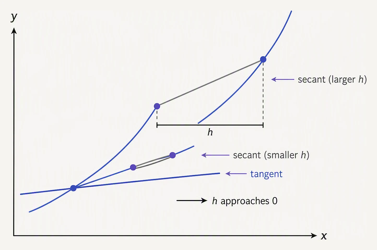
The derivative is the secant’s limit as the two points merge.
For a function f(x), the derivative f'(x) at a point x₀ is the
slope of the line tangent to the curve at that point. Equivalently,
it’s the best linear approximation of f near x₀:
f(x₀ + h) ≈ f(x₀) + f'(x₀) · h (for small h)Move a tiny bit h to the right. The function changes by approximately
f'(x₀) · h. That’s the whole point. If f'(x₀) > 0 the function is
increasing; if < 0, decreasing; if = 0, you’re at a (locally) flat
spot — maybe a minimum.
Drag the point — read the slope off the tangent line
The secant line touches the curve at two points a distance h apart. Shrink h toward 0 and watch it rotate into the tangent: that limiting slope is the derivative f′(x).
The formal definition makes the “zoom in” idea precise. Take a second
point a distance h away, draw the line through both — the secant — and
let h shrink to zero:
f'(x) = lim   (f(x + h) − f(x)) / h
        h→0
The secant slope (f(x+h) − f(x)) / h is the average rate of change over
that gap; the limit is the instantaneous rate at the point. Drag the
point above and animate h → 0 to watch the secant rotate into the
tangent.
Numerical derivative — the definition, on a computer
The textbook definition is the limit as h → 0 of
(f(x + h) - f(x)) / h. On a computer, just pick a small h:
import numpy as np

def f(x):
    return x**2

def numerical_derivative(f, x, h=1e-5):
    return (f(x + h) - f(x - h)) / (2 * h)    # symmetric -- more accurate

x0 = 3.0
slope = numerical_derivative(f, x0)
print(f"f(x) = x^2, slope at x={x0}: {slope:.4f}")
print(f"Exact analytical slope (2x): {2 * x0:.4f}")
f(x) = x^2, slope at x=3.0: 6.0000
Exact analytical slope (2x): 6.0000The “symmetric” version (f(x+h) - f(x-h)) / (2h) is the one to know —
it cancels the leading error term and gives much better accuracy. This
trick is the basis of “gradient checking” — comparing your hand-coded
gradient against a numerical one is a standard sanity check for ML
research code.
The handful of rules you actually use
You don’t need to memorize a table of 50. In ML, you’ll see roughly these:
d/dx [c]         = 0                  (constants don't change)
d/dx [x^n]       = n · x^(n-1)        (power rule)
d/dx [e^x]       = e^x                (exp is its own derivative)
d/dx [ln(x)]     = 1/x                (log is the inverse of exp)
d/dx [a · f(x)]  = a · f'(x)          (constants pull out)
d/dx [f(x)+g(x)] = f'(x) + g'(x)      (sum rule)
d/dx [f(g(x))]   = f'(g(x)) · g'(x)   (chain rule — the big one)
The chain rule is the only one you’ll lean on heavily. Backprop is the chain rule applied to a computational graph — that’s the next lesson.
Plot a function and its derivative
The clearest way to see a derivative is to plot both side by side. Where the function slopes up, the derivative is positive. Where it dips, the derivative is negative. At flat points (extrema), the derivative crosses zero.
import numpy as np
import matplotlib.pyplot as plt

x = np.linspace(-3, 3, 200)
f = x**3 - 3 * x                     # has a local max and a local min
fp = 3 * x**2 - 3                    # analytical derivative

fig, axes = plt.subplots(1, 2, figsize=(9, 3.5))
axes[0].plot(x, f)
axes[0].axhline(0, color="gray", lw=0.5)
axes[0].set_title("f(x) = x^3 - 3x")
axes[0].set_xlabel("x")

axes[1].plot(x, fp, color="orange")
axes[1].axhline(0, color="gray", lw=0.5)
axes[1].set_title("f'(x) = 3x^2 - 3")
axes[1].set_xlabel("x")

# Mark where derivative = 0
zeros = np.array([-1, 1])
for z in zeros:
    axes[0].axvline(z, ls=":", color="red", alpha=0.5)
    axes[1].axvline(z, ls=":", color="red", alpha=0.5)

plt.tight_layout()
plt.show()
print("Derivative is zero at x = -1 and x = +1 -- exactly the bumps of f.")
Derivative is zero at x = -1 and x = +1 -- exactly the bumps of f.The plot (plt.show()) draws f on the left and f' on the right, and the red dashed lines at x = -1 and x = +1 mark where f'(x) = 0 — exactly the local maximum and local minimum of f. Every optimization algorithm in ML is hunting for those zeros of the derivative.
Why derivatives matter for ML
A loss function L(w) takes parameters w and returns a number — how
wrong the model is. To minimize it, you want to find w where L'(w) = 0
(and where it’s a minimum, not a maximum or saddle).
For complicated L, you can’t solve L'(w) = 0 algebraically. Instead:
- Compute the derivative
L'(w)at your currentw. - Step in the direction that decreases
L— that’s-L'(w). - Repeat.
That’s gradient descent. The derivative is the only thing it needs.
# One-dimensional gradient descent on f(w) = (w - 3)^2.
import numpy as np

def f(w):  return (w - 3) ** 2
def fp(w): return 2 * (w - 3)

w = 0.0
lr = 0.1
for step in range(20):
    print(f"step {step:>2}  w={w:.4f}  f(w)={f(w):.4f}  f'(w)={fp(w):.4f}")
    w = w - lr * fp(w)
step 0 w=0.0000 f(w)=9.0000 f'(w)=-6.0000
step 1 w=0.6000 f(w)=5.7600 f'(w)=-4.8000
step 2 w=1.0800 f(w)=3.6864 f'(w)=-3.8400
step 3 w=1.4640 f(w)=2.3593 f'(w)=-3.0720
step 4 w=1.7712 f(w)=1.5099 f'(w)=-2.4576
step 5 w=2.0170 f(w)=0.9664 f'(w)=-1.9661
step 6 w=2.2136 f(w)=0.6185 f'(w)=-1.5729
step 7 w=2.3709 f(w)=0.3958 f'(w)=-1.2583
step 8 w=2.4967 f(w)=0.2533 f'(w)=-1.0066
step 9 w=2.5973 f(w)=0.1621 f'(w)=-0.8053
step 10 w=2.6779 f(w)=0.1038 f'(w)=-0.6442
step 11 w=2.7423 f(w)=0.0664 f'(w)=-0.5154
step 12 w=2.7938 f(w)=0.0425 f'(w)=-0.4123
step 13 w=2.8351 f(w)=0.0272 f'(w)=-0.3299
step 14 w=2.8681 f(w)=0.0174 f'(w)=-0.2639
step 15 w=2.8944 f(w)=0.0111 f'(w)=-0.2111
step 16 w=2.9156 f(w)=0.0071 f'(w)=-0.1689
step 17 w=2.9324 f(w)=0.0046 f'(w)=-0.1351
step 18 w=2.9460 f(w)=0.0029 f'(w)=-0.1081
step 19 w=2.9568 f(w)=0.0019 f'(w)=-0.0865Watch f'(w) shrink toward zero as w climbs toward 3, and the steps shorten with it — each move is lr · f'(w), so a gentler slope means a smaller step. When the derivative reaches zero you have stopped moving: you are at the minimum.
In one breath
A derivative f'(x) is the slope of a curve at one point — the best local linear fit, f(x₀ + h) ≈ f(x₀) + f'(x₀)·h. You can compute it on a computer with the symmetric difference (f(x+h) − f(x−h))/(2h), or from a small handful of rules (power, exp, log, sum, and above all the chain rule, which becomes backprop). A zero derivative marks a locally flat point — a candidate minimum — and since you usually cannot solve L'(w) = 0 directly, you instead step downhill along −L'(w) and repeat. That repetition is gradient descent, and the derivative is the only thing it needs.
Practice
Quick check
(f(x+h) - f(x-h)) / (2h). Why is it preferred over (f(x+h) - f(x)) / h?A question to carry forward
Everything above lived on a single knob: one input x, one slope f'(x), one number telling you which way to step — and on the toy (w − 3)² it worked beautifully. But a real loss does not have one knob. A linear regression has a handful; a neural network has millions — L(w₁, w₂, …, w_million) — and “the slope” is no longer a single number, because now you can move in a million directions at once.
So here is the thread onward: when a function has many inputs, what does its “slope” even mean? How do you take a derivative with respect to one parameter while a million others look on, what do you get when you stack all those slopes into a single vector — the gradient — and why does that one vector point in the exact direction that makes the loss climb fastest, so that stepping the opposite way is how everything in machine learning trains?
Practice this in an interview
All questionsBackpropagation uses the chain rule to compute the gradient of a scalar loss with respect to every model parameter by traversing the computation graph backward. It reuses intermediate gradients, making one forward pass and one backward pass far cheaper than calculating each parameter's gradient independently.
The vanishing gradient problem occurs when repeated Jacobian and derivative products make gradients shrink toward zero as they travel backward, so early layers barely learn. Common remedies are non-saturating hidden activations, suitable initialization, normalization, residual connections, and architectures with shorter or additive gradient paths.
Backpropagation computes the gradient of the loss with respect to every weight and bias by applying the chain rule backward through the network and reusing values from the forward pass. An optimizer then uses those gradients, usually by subtracting a scaled gradient, to update the parameters.
Vanilla SGD updates weights by a fixed fraction of the current gradient and oscillates badly in narrow loss valleys. Momentum accumulates a velocity vector that dampens oscillation and accelerates in consistent directions. RMSProp divides the learning rate by a running average of squared gradients per parameter, preventing large-gradient dimensions from dominating and stabilising training on non-stationary objectives.