Probability basics for ML
A random variable, the rules of probability, independence, conditioning, expectations. The ideas behind every classifier output and every A/B test.
Written and reviewed by Shreyash Prashu Last reviewed
What you'll learn
- Random variables and the rules every probability obeys
- Independence and conditional probability — the difference matters
- Expected value as a weighted average
- How to simulate probabilities in NumPy when you can't derive them
Before you start
The calculus chapter taught us to minimise a loss, then left a crack wide open: it never said where the loss came from. It also never said what to do when the data is random rather than fixed.
This chapter fills that gap, and it starts at the foundation. Every model that outputs a number between 0 and 1 — a fraud detector, an ad-click predictor, a medical-test classifier — is making a probability claim. Examples include:
- a fraud detector;
- an ad-click predictor;
- a medical-test classifier.
The same is true of:
- every A/B-test summary;
- every Bayesian prior;
- every cross-entropy loss;
- every confidence interval.
Understand probability and all of it stops being incantation. This lesson is the smallest set of ideas you cannot skip.
A random variable is just an outcome label
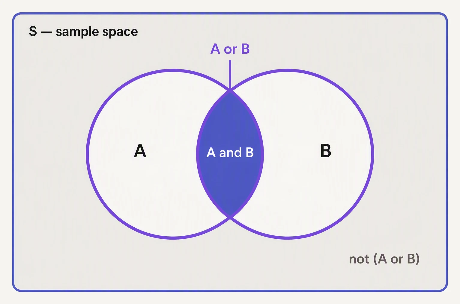
Everything else in probability is bookkeeping on top of this picture.
A random variable (a variable whose value is determined by a random process, not fixed in advance) lets us attach probabilities to outcomes.
Examples:
X = the result of a coin flip—Xtakes valueheadsortailswith some probability.Y = number of users who click an ad in the next minute.Z = a draw from a normal distribution.
The variable stands in for “I don’t know what value will come out, but I know the distribution of possible values.”
The three rules
0 ≤ P(event) ≤ 1— probabilities live in [0, 1].P(everything) = 1— something has to happen.- For disjoint events,
P(A or B) = P(A) + P(B).
These three rules are the entire foundation. Everything else is a consequence.
Sum-to-one for a discrete distribution:
import numpy as np

# Distribution over dice outcomes
faces = np.arange(1, 7)
probs = np.array([1/6] * 6)

print("Faces:", faces)
print("P(face):", probs.round(3))
print("Sum of all probabilities:", probs.sum())     # ~1.0

# P(rolling 3 or higher) = P(3) + P(4) + P(5) + P(6)
print("P(>= 3):", probs[faces >= 3].sum())
Faces: [1 2 3 4 5 6]
P(face): [0.167 0.167 0.167 0.167 0.167 0.167]
Sum of all probabilities: 0.9999999999999999
P(>= 3): 0.6666666666666666The six probabilities sum to 0.9999999999999999 — floating-point’s honest way of writing 1 (six copies of 1/6 cannot be stored exactly in binary). Rule 2 holds; the tiny error is the computer, not the math.
And P(≥ 3) = 4/6 = 0.667 is rule 3 in action: four disjoint faces, probabilities added.
Flip, roll, watch theory meet practice
Independence: P(A and B) = P(A) · P(B)
Two events are independent if knowing one happened doesn’t change the probability of the other.
Examples include:
- Coin flips.
- Different dice.
- Different users (usually) clicking on an ad.
When events are independent, joint probabilities multiply:
P(A ∩ B) = P(A) · P(B)A famous gotcha: two events that are individually likely can still have a tiny joint probability if you need them both to happen.
# P(any single die rolls a 6) = 1/6 ≈ 0.167
# P(5 dice ALL roll 6) = (1/6)^5 -- vanishingly small
print("Single die six:", 1/6)
print("All five sixes:", (1/6) ** 5)
print("Roughly 1 in", round(6 ** 5))
Single die six: 0.16666666666666666
All five sixes: 0.00012860082304526745
Roughly 1 in 7776One six is a coin-toss-ish 0.167. Five independent sixes multiply down to 0.000129 — about 1 in 7,776.
Multiplying probabilities shrinks them fast, which is exactly why a model that needs all of several conditions to hold at once succeeds so rarely.
Conditional probability: P(A | B)
P(A | B) reads as “probability of A given B.” It’s how much you should believe A happens if you already know B happened. Defined as:
P(A | B) = P(A ∩ B) / P(B)Cool fact: if A and B are independent, P(A | B) = P(A) — knowing B adds no information. If they’re not independent, conditioning shifts the probability.
Drag the events — conditioning shrinks the universe
Click-through example. Suppose:
- P(user clicks an ad) = 2% overall.
- P(user clicks | user is “high intent” segment) = 8%.
Those numbers are very different. The “given the segment” version is what you’d actually use to predict.
# Suppose we have a user segment table.
# Out of 10,000 users, 1,500 are "high intent" -- and 120 of those clicked.
# Among the other 8,500, only 80 clicked.

high_intent = 1500
high_clicks = 120
other = 8500
other_clicks = 80

total = high_intent + other
total_clicks = high_clicks + other_clicks

print(f"P(click) overall:               {total_clicks/total:.4f}")
print(f"P(click | high intent):         {high_clicks/high_intent:.4f}")
print(f"P(click | NOT high intent):     {other_clicks/other:.4f}")
print(f"P(high intent | click):         {high_clicks/total_clicks:.4f}")
P(click) overall: 0.0200
P(click | high intent): 0.0800
P(click | NOT high intent): 0.0094
P(high intent | click): 0.6000Conditioning on the segment moves the number a long way: a 2% overall click rate becomes 8% once you know the user is high-intent. It falls to under 1% if they are not.
That gap is the whole reason segmentation works.
Notice the last line — P(high intent | click) flips the question around. P(A | B) and P(B | A) are not the same thing.
Confusing them (base rate neglect) is one of the most common reasoning errors in:
- medicine;
- security;
- ML monitoring.
Bayes’ theorem is the formal tool for flipping conditionals correctly. That deserves its own lesson, but the seed is right here.
Expected value: the weighted average
The expected value of a random variable — the probability-weighted average of all possible outcomes — is the average you’d get if you ran the experiment infinitely many times. For a discrete random variable:
E[X] = Σ x · P(X = x) (weighted sum over outcomes)For a dice roll: E[X] = 1·(1/6) + 2·(1/6) + ... + 6·(1/6) = 3.5.
Not a value the die can actually land on — but it’s the long-run average.
import numpy as np

# Analytical expectation
faces = np.arange(1, 7)
probs = np.ones(6) / 6
expected = (faces * probs).sum()
print("E[die roll] analytical:", expected)

# Verify via simulation: average of many rolls converges
rng = np.random.default_rng(0)
rolls = rng.integers(1, 7, size=100_000)
print("E[die roll] simulated:  ", rolls.mean())
E[die roll] analytical: 3.5
E[die roll] simulated: 3.49798The formula gives 3.5 exactly. A hundred thousand simulated rolls average 3.49798 — close enough to confirm it, and a first taste of the law of large numbers.
The empirical mean homes in on the expected value as the sample grows.
Expected value is everywhere in ML. It’s the math behind:
- the expected loss that training minimizes;
- the reward that reinforcement learning maximizes;
- the conversion rate the A/B test estimates.
Simulation: when math is too hard, sample
The thing that makes NumPy a superpower for probability: you can estimate any probability by sampling the underlying process.
Imagine you ask: “If I flip a fair coin 10 times, what’s the probability of getting exactly 7 heads?”
You could compute it from the binomial formula. Or you could simulate:
import numpy as np

rng = np.random.default_rng(0)

n_trials = 100_000          # simulate 100k experiments
n_flips = 10

# Each row is one experiment of 10 flips. 1 = heads, 0 = tails.
flips = rng.integers(0, 2, size=(n_trials, n_flips))
heads_per_trial = flips.sum(axis=1)

p_exactly_7 = (heads_per_trial == 7).mean()
print(f"P(exactly 7 heads in 10 flips): {p_exactly_7:.4f}")

# True analytical value:
from math import comb
true = comb(10, 7) * (0.5) ** 10
print(f"True value:                    {true:.4f}")
P(exactly 7 heads in 10 flips): 0.1195
True value: 0.1172The simulation lands at 0.1195 against the true 0.1172 — within a couple of thousandths, from nothing but counting how often 7 heads showed up across 100,000 imagined experiments.
Monte Carlo simulation is the data scientist’s swiss army knife: when the math gets hairy, simulate.
In one breath
A random variable stands in for an outcome you cannot predict but whose distribution you know, and every probability obeys three rules: it lies in [0, 1], the total over all outcomes is 1, and disjoint events add.
Two events are independent when P(A∩B) = P(A)·P(B) — their joint probability multiplies, so five sixes in a row is (1/6)⁵.
Conditional probability P(A|B) = P(A∩B)/P(B) updates a belief once you know B, and crucially P(A|B) ≠ P(B|A) (the base-rate trap).
The expected value E[X] = Σ x·P(X=x) is the long-run weighted average — the math behind expected loss, RL reward, and a conversion rate.
And when the algebra gets hard, simulate: sample the process tens of thousands of times and read the probability straight off the frequency.
Practice
Quick check
A question to carry forward
One line in this lesson did something the rest did not. When we computed P(high intent | click) = 0.60, we flipped a conditional.
We started from “given the segment, how likely is a click?” and turned it into “given a click, how likely is the segment?” The disease quiz then drove the danger home: a test that is “90% accurate” still leaves a positive result only about half likely to be real, because the base rate was low.
P(A|B) and P(B|A) are genuinely different numbers, and quietly confusing them is one of the costliest reasoning errors in medicine, security, and ML monitoring alike.
So here is the thread onward: there is one exact formula for flipping a conditional the right way.
It turns P(evidence | hypothesis), which you can usually measure, into P(hypothesis | evidence), which you actually want. It weaves the base rate in so a low one never fools you again.
What is Bayes’ theorem, and why is it less a formula than a complete recipe for updating belief in the light of evidence? How does that one update sit underneath:
- spam filters;
- medical diagnosis;
- the entire Bayesian view of machine learning?
Practice this in an interview
All questionsConditional probability P(A|B) is the probability of A after learning that B occurred, computed as P(A and B) divided by P(B). Joint probability P(A and B) is the probability that both events occur in the full sample space, so conditional probability changes the denominator while joint probability does not.
Expected value is the probability-weighted center of a random variable, while variance is the expected squared distance from that center. Expected value is always linear, but variance needs scaling and covariance terms; independence is only required for the familiar variance-addition shortcut.
Mutually exclusive events cannot both occur at once — knowing one happened tells you the other didn't. Independent events can both occur, but knowing one happened gives no information about the other. These concepts are nearly opposite: non-trivial mutually exclusive events are always dependent.
The joint distribution P(X, Y) fully specifies two random variables together. Marginals P(X) and P(Y) are obtained by summing (or integrating) the joint over the other variable. Conditionals P(X|Y=y) are the joint sliced at a fixed y value, renormalized by the marginal P(Y=y).
In the Monty Hall problem, a host who knows where the prize is always opens an empty door — this action transfers probability mass to the remaining unopened door, making switching win with probability 2/3 and staying win only 1/3. The key is that the host's action is not random.
The main probability sampling methods are simple random sampling, stratified sampling, cluster sampling, and systematic sampling. Bias enters when some units have a zero or systematically different probability of selection — as in convenience sampling, survivorship bias, or non-response bias — making the sample unrepresentative of the target population regardless of size.