The Central Limit Theorem
Average enough independent samples — from ANY distribution — and the result is normal. This is the proof behind the bell curve's ubiquity, and the reason A/B tests, confidence intervals, and t-tests all work.
Written and reviewed by Shreyash Prashu Last reviewed
What you'll learn
- The CLT in words: averages of independent samples go normal, whatever the original shape
- Why the underlying distribution doesn't have to be normal — and the cancellation that does it
- The two numbers it pins down: the mean μ and the spread σ/√n
- How fast convergence happens (n = 30 is folklore, not law)
- The CLT's role in confidence intervals and hypothesis tests
Before you start
We have been quietly running up a debt. Twice now — once for the bell curve, once for its many-dimensional cousin — we reached for the Gaussian and waved at the same excuse: “because of the Central Limit Theorem.” A reason you keep citing but never prove is a loan, and this lesson pays it back in full.
Here is the claim, and it is strange enough to deserve a little suspicion. Take any
distribution at all — a lopsided die, a skewed stream of incomes, the wait between two buses, a
single coin flip. Draw n independent samples from it and average them. Save that average.
Do it again, and again, thousands of times. The pile of averages you collect is not lopsided,
not skewed, not two-valued. It is a smooth, symmetric bell — and it grows more bell-shaped
the larger n gets. The shape you started from barely leaves a fingerprint.
That single fact is the Central Limit Theorem (CLT). It is the reason normal-distribution machinery — z-scores, t-tests, confidence intervals — works on data that is nothing like a bell curve.
The statement, in plain English
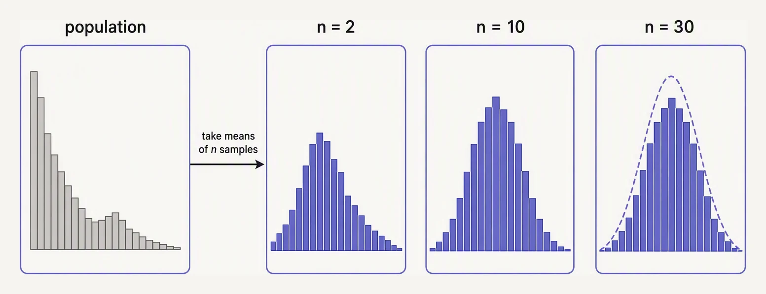
The population can be any shape. The distribution of its means still goes normal.
Pick a distribution. It can be uniform, exponential, wildly skewed, discrete — anything, as long as it has a finite variance. Now repeat three steps many times:
- Draw
nindependent samples. - Compute their mean.
- Save that mean.
The collection of saved means has its own distribution — the sampling distribution of the
mean — and as n grows it approaches a normal with two pinned-down numbers:
mean    = μ            (the true mean of the original distribution)
std dev = σ / √n       (its true std dev, shrunk by √n)
Why does a bell fall out, no matter where you started? Picture the mean as a tug-of-war. Each
sample chips in its own little pull — some high, some low. Across n of them the extremes on one
side tend to be cancelled by extremes on the other, and what survives the cancellation piles up
symmetrically around the true centre. That laundering of idiosyncrasy into symmetry is the whole
mechanism, and the normal is the unique shape it converges to.
The √n is the workhorse half of the statement. Double your sample size and the noise does not
halve — it shrinks only by √2 ≈ 1.4. To genuinely halve the noise you need 4× the data. That
one line of arithmetic governs every A/B-test sample-size calculation you will ever run.
Average enough samples and you always get a bell
Pick a population — however lopsided — set a sample size n, then draw samples and watch their means pile up into a normal curve.
Watch it happen — starting from the exponential
The exponential distribution is heavily skewed: a long tail to the right, nothing to the left of
zero. If the CLT is true, averages of exponentials should still march toward a bell. Average n
of them, repeat 5000 times, and look at the histogram of those means as n climbs.
import numpy as np
import matplotlib.pyplot as plt

rng = np.random.default_rng(0)

# Original distribution: Exponential with mean 5 — clearly NOT normal.
# Average n samples, repeat 5000 times, and look at the histogram of those means.
n_trials = 5000
sample_sizes = [1, 5, 30, 100]

fig, axes = plt.subplots(1, 4, figsize=(13, 3.2), sharey=True)
for ax, n in zip(axes, sample_sizes):
    means = np.array([rng.exponential(scale=5.0, size=n).mean() for _ in range(n_trials)])
    ax.hist(means, bins=40, color="steelblue", density=True)
    ax.set_title(f"n = {n}\nmean={means.mean():.2f}, std={means.std():.2f}")
    ax.set_xlabel("sample mean")
    print(f"n = {n:>3}:  centre = {means.mean():.2f}   spread (std of the means) = {means.std():.2f}")
axes[0].set_ylabel("density")
plt.suptitle("Distribution of sample means: starts skewed, ends bell-shaped")
plt.tight_layout()
plt.show()
n = 1: centre = 5.07 spread (std of the means) = 5.14
n = 5: centre = 4.94 spread (std of the means) = 2.20
n = 30: centre = 4.99 spread (std of the means) = 0.93
n = 100: centre = 5.00 spread (std of the means) = 0.50The four panels tell the whole story. At n = 1 you are just staring at raw exponential samples
— a sharp peak near zero and a long right tail, skewed and ugly. At n = 5 the skew has already
started to soften. By n = 30 the histogram is, to the eye, a bell. At n = 100 you could not
tell it from a normal if you tried.
And notice the second column of numbers. The centre parks at 5.00 — the true mean μ — and
never drifts. The spread collapses on schedule: 5 / √100 = 0.5, exactly the σ/√n the
theorem promised. The shape becomes normal and the formula for its width is handed to you for
free.
Quantify the convergence
That σ/√n is not folklore — it is a number you can check to four decimals. Average an
exponential (μ = 5, and for the exponential σ = μ = 5) at a ladder of sample sizes, and
compare the observed spread of the means against the predicted σ/√n.
import numpy as np

rng = np.random.default_rng(0)

# Exponential with mean μ = 5, so std σ = 5 (for the exponential, σ = μ).
mu_true, sigma_true = 5.0, 5.0
n_trials = 50_000

for n in [1, 5, 30, 100, 1000]:
    means = np.array([rng.exponential(scale=mu_true, size=n).mean() for _ in range(n_trials)])
    predicted_std = sigma_true / np.sqrt(n)
    print(f"n={n:>4}   observed std of mean = {means.std():.4f}   predicted σ/√n = {predicted_std:.4f}")
n= 1 observed std of mean = 5.0253 predicted σ/√n = 5.0000
n= 5 observed std of mean = 2.2475 predicted σ/√n = 2.2361
n= 30 observed std of mean = 0.9068 predicted σ/√n = 0.9129
n= 100 observed std of mean = 0.5002 predicted σ/√n = 0.5000
n=1000 observed std of mean = 0.1584 predicted σ/√n = 0.1581
Observed and predicted agree to within sampling noise, every row. This is what lifts the CLT from a pretty shape result to a quantitative tool: it tells you not just that the means go normal, but exactly how tightly they will cluster.
What does “n = 30” actually mean?
You will hear “the CLT kicks in around n = 30” repeated as if it were law. It is not. How fast the convergence happens depends entirely on the distribution you started from.
- Already symmetric (uniform, a fair coin)? Even
n = 5looks close to normal. - Moderately skewed (exponential, a reasonable log-normal)?
n = 30is a decent rule. - Savagely heavy-tailed? You may need far more — and in the pathological Cauchy case
(infinite variance) the CLT does not apply at all, so even
n = 10,000never settles.
The rule of thumb is really a rule of skew: the more lopsided or heavy-tailed the population, the more samples you must average before the bell is a good approximation.
Why the CLT runs data science
Every confidence interval, every A/B test, every “is this difference significant?” leans on this one theorem. The pattern is always the same: you measure a sample, and you want to say something honest about the population it came from.
Take a conversion rate. You observe 10,000 users — each one a stark 0 or 1, about as un-normal
as data gets. Yet the CLT promises your sample mean (the observed rate) is approximately normal
around the true rate, with standard deviation σ/√n. That single promise hands you the
confidence-interval formula:
sample_mean ± 1.96 · σ / √n (95% confidence interval)The 1.96 is the 97.5th percentile of the standard normal — the number that fences in the middle
95% of a bell. Watch it fall straight out of a Bernoulli stream:
import numpy as np

rng = np.random.default_rng(0)

# True conversion rate is 5%. We measure n = 10,000 users.
n = 10_000
p_true = 0.05
sample = rng.binomial(1, p_true, size=n)
p_hat = sample.mean()

# Standard error: for a proportion, σ/√n = √(p(1-p)/n)
se = np.sqrt(p_hat * (1 - p_hat) / n)
lo = p_hat - 1.96 * se
hi = p_hat + 1.96 * se

print(f"Observed conversion: {p_hat:.4f}")
print(f"95% confidence interval: [{lo:.4f}, {hi:.4f}]")
print(f"(True rate {p_true} should sit inside this interval ~95% of the time across reruns)")
Observed conversion: 0.0498
95% confidence interval: [0.0455, 0.0541]
(True rate 0.05 should sit inside this interval ~95% of the time across reruns)That interval is literally the CLT in action. The 1.96 comes from normality; the √n in the
standard error comes from the variance-shrinking rule. Strip the CLT away and the whole apparatus
of statistical inference loses its foundation.
In one breath
The Central Limit Theorem says that if you draw n independent samples from any distribution
with finite variance, average them, and repeat, the distribution of those averages — the sampling
distribution of the mean — approaches a normal, centred at the true mean μ with spread
σ/√n, no matter how un-normal the original was. The mechanism is cancellation: extremes on
either side wash out, leaving a symmetric pile around the centre. It does not normalise your raw
data — only the averages. The √n law (halving noise costs 4× the data) and the 1.96 of a 95%
interval both come straight from it, which is why confidence intervals, A/B tests, and t-tests all
rest on this one result. Caveat: finite variance is required — heavy-tailed Cauchy breaks it
entirely.
Practice
Quick check
A question to carry forward
The CLT just made a promise about a whole cloud of sample means: average 200 users many times
and the averages form a tidy normal around the truth, spread by σ/√n. But step back into real
life and the promise has a catch. You do not get to rerun the experiment 5000 times. You get
one sample — 200 users, one mean of 4.2 minutes — and the true average you are chasing stays
forever out of sight.
So here is the thread onward. Given a single number squeezed out of a single sample, how do you
state honestly how far off it might be? What is an estimator, why is the σ/√n we just met
called its standard error, and how does it become a confidence interval — the most
quoted and most misunderstood object in all of statistics? (Ask yourself now: when someone reports
“95% confident the mean is between 4.0 and 4.4,” what exactly is the 95% a probability about? The
honest answer trips up almost everyone.)
Practice this in an interview
All questionsThe CLT states that the sampling distribution of the sample mean converges to a normal distribution as sample size grows, regardless of the shape of the underlying population distribution. It is the theoretical foundation for confidence intervals, hypothesis tests, and many machine-learning approximations — but it applies to the distribution of the mean, not to the raw data.
The Law of Large Numbers (LLN) says the sample mean converges to the true mean as sample size grows — it is a statement about where the mean lands. The Central Limit Theorem says the sampling distribution of the mean is approximately normal — it is a statement about the shape of that distribution. LLN guarantees convergence; CLT characterises the rate and shape of that convergence.
The Normal distribution is justified by the Central Limit Theorem — averages of large i.i.d. samples converge to Normal regardless of the underlying distribution. It is fully characterized by mean and variance, enabling closed-form inference. It fails for heavy-tailed data, skewed outcomes, bounded quantities, and rare extreme events.
Standard deviation measures the spread of individual observations around the population mean. Standard error measures the spread of sample means around the true mean — it equals the standard deviation divided by the square root of the sample size, so it shrinks as the sample grows while the standard deviation does not.