Rank, linear independence, span & basis
When does a feature add real information, and when is it just a copy of the others? Span, independence, basis, and rank are the four ideas that answer it — and they decide whether your model can even be fit.
What you'll learn
- Span — the set of everything you can build from a group of vectors
- Linear independence — when no vector is redundant
- Basis & dimension — a minimal coordinate system for a space
- Rank — the number of independent directions, and how it ties RREF, SVD, and regression together
- Why rank deficiency (multicollinearity) breaks models and how to spot it
Before you start
The last lesson left rank as a cliffhanger: a single integer — the pivot count — that
silently decided whether Ax = b had one solution, many, or none. But “pivots left after
elimination” describes how to compute rank, not what it is. Here is what it is, told
through the smallest example there is. You add a “price in dollars” column and a “price in
cents” column to your dataset; the second carries zero new information — it is just the
first times 100. Linear algebra has exact words for that redundancy, and those words decide
whether your model can be fit at all.
Span: what you can reach
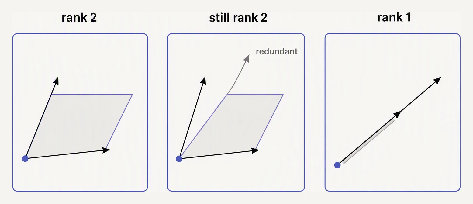
Rank counts genuinely new directions, not how many vectors you were handed.
The span of a set of vectors is every point you can reach by scaling
and adding them: all combinations a·v₁ + b·v₂ + …. Two vectors pointing
in different directions span the whole 2D plane. Two vectors on the same
line span only that line.
Linear independence: is anyone redundant?
A set is linearly independent if no vector can be built from the others — equivalently, the only way to combine them into the zero vector is to multiply them all by zero. The moment one vector is a combination of the rest, the set is dependent, and that vector adds nothing to the span.
Independent. Their combinations fill the whole plane — together they're a basis for ℝ².
Drag either arrowhead. Rank = the number of independent directions = the dimension of the span.
Basis & dimension
A basis is the sweet spot: a set that is independent and spans
the space — a minimal, non-redundant coordinate system. The number of
vectors in a basis is the dimension of the space. ℝ² needs exactly
two; any third vector is necessarily dependent.
Rank: the number that ties it all together
The rank of a matrix is the number of linearly independent columns — equivalently, the dimension of the space its columns span. And it shows up everywhere you’ve already been:
- It’s the number of pivots in the RREF (last lesson).
- It’s the number of non-zero singular values in the SVD (next idea).
- A square matrix is invertible iff it has full rank.
import numpy as np

# price_dollars, price_cents (= 100x), and a genuinely new feature
dollars = np.array([3., 5., 2., 9.])
X = np.column_stack([dollars, dollars * 100, [1., 0., 1., 1.]])

print("shape:", X.shape, " columns:", X.shape[1])
print("rank :", np.linalg.matrix_rank(X))   # 2, not 3 -- one column is redundant

# Rank deficiency => XtX is singular => no unique least-squares solution
XtX = X.T @ X
print("det(XᵀX):", round(np.linalg.det(XtX), 6))   # ~0 -> singular
shape: (4, 3) columns: 3
rank : 2
det(XᵀX): 0.0Three columns, but rank 2 — the “cents” column is dependent, so it adds a
direction the data already had. XᵀX becomes singular and the normal
equations lose their unique solution.
Where this lives in ML
- Multicollinearity. Correlated features make the feature matrix near-rank-deficient. Coefficients become unstable and uninterpretable — the model can’t decide how to split credit between the copies.
- The dummy-variable trap. One-hot encode a category into k columns and include an intercept, and the columns sum to a constant — instant linear dependence. That’s why you drop one level.
- Effective dimensionality. Your data may live in 300 columns but have rank 12 — only 12 directions of real variation. That’s the gap PCA and SVD exploit.
In one breath
Four ideas pin down “redundant information.” The span of a set of vectors is everything you can build from them by scaling and adding; a set is linearly independent when no vector is a combination of the others (no one is redundant); a basis is the sweet spot — independent and spanning, a minimal coordinate system whose size is the space’s dimension; and the rank of a matrix is the number of independent columns — the same number as the pivots in its RREF and the non-zero singular values in its SVD. When rank < number of columns (multicollinearity, the dummy-variable trap), XᵀX is singular and the fit has no unique answer — and that same gap is what PCA and SVD exploit when 300 columns really carry only 12 directions.
Practice
Quick check
A question to carry forward
Rank told us how many independent directions a set of columns truly has. But it stayed silent on a softer, more useful question: not merely whether two directions are independent, but whether they are independent in the cleanest way — at right angles, each casting no shadow on the other at all. When the columns of a matrix are mutually perpendicular, a surprising number of hard problems collapse into easy ones.
And that matters most exactly where rank just stranded us. When Ax = b has no exact solution — too many noisy equations, too few unknowns, the everyday reality of regression — we cannot solve it, but we can ask for the next best thing: the x that comes closest. Here is the thread onward: what does “closest” mean geometrically — a projection, a perpendicular dropped onto the space the columns span — why does orthogonality make that closest answer almost effortless to compute, and how is this single idea, least squares, the exact engine that fits a straight line through a cloud of scattered points?
Practice this in an interview
All questionsThe usual five assumptions are linearity, independent errors, constant error variance, normal residuals for exact small-sample inference, and no perfect multicollinearity; a technically complete answer also requires zero conditional mean. Each violation harms a different part of OLS: fit and bias, efficiency, standard errors, inference, or coefficient identifiability.
Scale features for distance-based models, PCA, neural networks, and regularized linear or logistic models because magnitudes affect geometry, optimization, or coefficient penalties. Tree-based models generally do not need scaling because threshold splits preserve feature order; ordinary unregularized linear models may work without it, but scaling often improves numerical conditioning.
Multicollinearity means predictors carry overlapping linear information, so ordinary least squares estimates individual coefficients with high variance even when predictions remain accurate. Detect it with correlation checks, VIF, and condition diagnostics; address it by removing or combining redundant features, collecting more informative data, or using regularization such as ridge when prediction matters more than coefficient interpretation.
Standardization rescales features to zero mean and unit variance; normalization squashes values into a fixed range, usually [0, 1]. Distance-based and gradient-based models are sensitive to scale and require one of these; tree-based models split on rank order and are scale-invariant.