Partial derivatives and the gradient
When a loss has many parameters, you take a derivative with respect to each one. Stack them into a vector and you have the gradient — the heart of training.
Written and reviewed by Shreyash Prashu Last reviewed
What you'll learn
- What it means to take a derivative "with respect to one variable"
- The gradient as the vector of all partial derivatives
- The geometric reading — each partial is a slope in one axis direction
- How loss gradients drive every weight update in a neural net
Before you start
The last lesson left us with one knob and a worry: a real loss has a million of them. What becomes of “the slope” when you can move in a million directions at once?
The answer is disarmingly simple. Take the derivative with respect to one variable at a time, treating every other as a frozen constant. Each of those is a partial derivative. Then pack them into a single vector and you have the gradient, the multivariable generalisation of slope and the one quantity every weight update in deep learning is built on.
Partial derivative: pin everything else
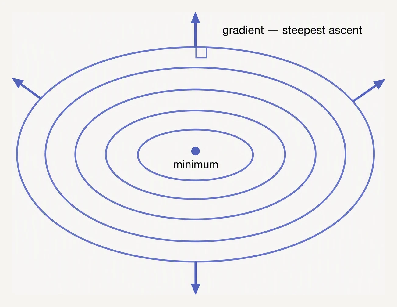
The gradient is perpendicular to the contour and points straight uphill.
For f(x, y), the partial derivative with respect to x is written
∂f/∂x. The notation switches from d to ∂ to remind you that other
variables are still around — you’re just freezing them.
Example: f(x, y) = x² + 3xy + y³.
∂f/∂x  = 2x + 3y       (y is a constant for this calculation)
∂f/∂y  = 3x + 3y²      (x is a constant for this calculation)
That’s the whole technique. There is no extra calculus to learn.
Geometric reading: slope along an axis
∂f/∂x is the slope you’d feel if you stood at (x₀, y₀) and walked
in the positive x direction, holding y fixed. ∂f/∂y is the slope
if you walked in the positive y direction.
Imagine f(x, y) as a landscape — a surface above the xy-plane. Stand
on it. Looking east-west gives you one slope (∂f/∂x). Looking
north-south gives you another (∂f/∂y). Together they tell you the
shape of the local terrain.
The gradient is the stack
The gradient of f is the vector of all partials:
∇f(x, y) = [ ∂f/∂x, ∂f/∂y ]For the example above:
∇f(x, y) = [ 2x + 3y, 3x + 3y² ]At a specific point, say (1, 2):
∇f(1, 2) = [ 2 + 6, 3 + 12 ] = [ 8, 15 ]That vector has two readings:
- Direction —
∇fpoints in the directionfincreases fastest. - Magnitude —
||∇f||is how steep that fastest-uphill direction is.
Why is ∇f the steepest direction? The rate of change of f in any
unit direction u is ∇f · u (the dot product). This is maximized when
u is parallel to ∇f — that’s a basic property of the dot product.
Every other direction gives a smaller increase. So ∇f is, by definition,
the steepest uphill direction.
To minimize f you step in -∇f. That’s exactly what gradient descent
does.
Drag the point — see ∂f/∂x and ∂f/∂y as the gradient's components
The gradient ∇f is the diagonal of the rectangle formed by ∂f/∂x and ∂f/∂y. Gradient descent steps in −∇f.
A simple quadratic, computed
import numpy as np

# f(x, y) = x^2 + 3xy + y^3
def f(x, y):
    return x**2 + 3 * x * y + y**3

def grad(x, y):
    return np.array([2 * x + 3 * y, 3 * x + 3 * y**2])

print("f(1, 2) =", f(1, 2))
print("grad f(1, 2) =", grad(1, 2))

# Numerical check via central differences
def num_partial(f, x, y, var, h=1e-5):
    if var == "x":
        return (f(x + h, y) - f(x - h, y)) / (2 * h)
    else:
        return (f(x, y + h) - f(x, y - h)) / (2 * h)

print("df/dx numerically:", num_partial(f, 1, 2, "x"))
print("df/dy numerically:", num_partial(f, 1, 2, "y"))
f(1, 2) = 15
grad f(1, 2) = [ 8 15]
df/dx numerically: 7.999999999963591
df/dy numerically: 15.000000000231493The numerical partials land on 7.9999… and 15.0000… — the central-difference approximation of the exact [8, 15], off only in the last few digits. Analytical and numerical agree; the gradient is confirmed.
Visualizing a 2D gradient field
For f(x, y) = x² + 3y², the minimum is at (0, 0). The gradient at
each point should point away from the origin. Let’s see it.
import numpy as np
import matplotlib.pyplot as plt

# f(x, y) = x^2 + 3y^2 -- tilted bowl, min at (0,0)
xs = np.linspace(-3, 3, 20)
ys = np.linspace(-2, 2, 15)
X, Y = np.meshgrid(xs, ys)

# Gradient: grad f = [2x, 6y]
U = 2 * X
V = 6 * Y
print("sample gradient at (1, 1): [2x, 6y] =", [2 * 1, 6 * 1])

# Contours of f underneath
xs_fine = np.linspace(-3, 3, 100)
ys_fine = np.linspace(-2, 2, 100)
Xf, Yf = np.meshgrid(xs_fine, ys_fine)
Zf = Xf**2 + 3 * Yf**2

fig, ax = plt.subplots(figsize=(7, 4))
ax.contour(Xf, Yf, Zf, levels=10, alpha=0.4)
ax.quiver(X, Y, U, V, color="steelblue", scale=80)
ax.scatter([0], [0], color="red", zorder=5, label="minimum")
ax.set_title("Gradient of f(x,y) = x^2 + 3y^2")
ax.set_xlabel("x"); ax.set_ylabel("y")
ax.legend()
plt.tight_layout()
plt.show()
sample gradient at (1, 1): [2x, 6y] = [2, 6]The plot (plt.show()) draws the bowl’s contours with a gradient arrow at every grid point. Each arrow points uphill, away from the minimum at the origin, and grows longer where the bowl is steeper.
Gradient descent simply flips every arrow around and walks the other way, toward the bottom.
Why this matters for ML: loss gradients
A neural net’s loss L(w) is a function of millions of weights. To
update each weight, you need ∂L/∂w_i — the partial derivative of the
loss with respect to that one weight. The gradient ∇L collects all
of these into one big vector.
The update rule applies it weight-by-weight:
w_i ← w_i - lr * ∂L/∂w_i # for every parameter iIn vector form:
w ← w - lr * ∇L(w)Same equation, one is element-wise, the other is the whole vector at once.
# A tiny multivariate optimization: minimize L(w) = (w[0] - 2)^2 + 3 * (w[1] + 1)^2
import numpy as np

def L(w):
    return (w[0] - 2)**2 + 3 * (w[1] + 1)**2

def grad_L(w):
    return np.array([2 * (w[0] - 2),  6 * (w[1] + 1)])

w = np.array([0.0, 0.0])
lr = 0.1

for step in range(20):
    g = grad_L(w)
    print(f"step {step:>2}  w={w}  L={L(w):.4f}  ||grad L||={np.linalg.norm(g):.4f}")
    w = w - lr * g

print(f"\nConverged to w = {w}  (true minimum: [2, -1])")
step 0 w=[0. 0.] L=7.0000 ||grad L||=7.2111
step 1 w=[ 0.4 -0.6] L=3.0400 ||grad L||=4.0000
step 2 w=[ 0.72 -0.84] L=1.7152 ||grad L||=2.7341
step 3 w=[ 0.976 -0.936] L=1.0609 ||grad L||=2.0837
step 4 w=[ 1.1808 -0.9744] L=0.6731 ||grad L||=1.6456
step 5 w=[ 1.34464 -0.98976] L=0.4298 ||grad L||=1.3122
... (steps 6-9, 11-14, 16-18 omitted)
step 10 w=[ 1.78525164 -0.99989514] L=0.0461 ||grad L||=0.4295
step 15 w=[ 1.92963126 -0.99999893] L=0.0050 ||grad L||=0.1407
step 19 w=[ 1.97117696 -0.99999997] L=0.0008 ||grad L||=0.0576
Converged to w = [ 1.97694157 -0.99999999] (true minimum: [2, -1])Watch the gradient norm shrink toward zero. Notice too that the second coordinate (with its steeper 3·(w₁+1)² bowl and gradient 6(w₁+1)) snaps to −1 almost immediately, while the gentler first coordinate is still inching toward 2 at step 19.
This is a first glimpse of how uneven curvature slows plain gradient descent.
In one breath
A partial derivative ∂f/∂x is an ordinary derivative taken with respect to one variable while every other is pinned as a constant — no new calculus to learn.
Stack all the partials into a vector and you have the gradient ∇f, which carries two readings:
- It points in the direction
fincreases fastest. The rate of change along any unit directionuis∇f · u, maximised whenu ‖ ∇f. - Its length
‖∇f‖is how steep that climb is.
To minimise, step along −∇f: w ← w − lr·∇L(w), applied to all million weights at once.
That single update — with ∇L computed for you by autograd’s loss.backward() — is how every neural network learns.
Practice
Quick check
A question to carry forward
We now hold the gradient and, almost in passing, the rule that uses it — w ← w − lr·∇L(w): take the steepest-downhill direction and step. We even watched it crawl a toy loss to its minimum.
But we waved past the one symbol that decides whether any of it works: that lr, the learning rate, the length of each step.
Make it too small and training drags on forever; too large and the steps overshoot the valley, bounce up the far wall, and the loss explodes instead of shrinking.
And real loss landscapes are nothing like our tidy bowls — they have ravines, plateaus, and saddle points that can stall the walk entirely (you already glimpsed it: one coordinate raced to its answer while the other crawled).
Here is the thread onward: gradient descent earns a lesson of its own. It asks three questions:
- How do you choose the step size?
- What do momentum and the adaptive optimizers behind every real model actually fix?
- What separates a descent that converges from one that diverges?
Practice this in an interview
All questionsBackpropagation uses the chain rule to compute the gradient of a scalar loss with respect to every model parameter by traversing the computation graph backward. It reuses intermediate gradients, making one forward pass and one backward pass far cheaper than calculating each parameter's gradient independently.
Backpropagation computes the gradient of the loss with respect to every weight and bias by applying the chain rule backward through the network and reusing values from the forward pass. An optimizer then uses those gradients, usually by subtracting a scaled gradient, to update the parameters.
The vanishing gradient problem occurs when repeated Jacobian and derivative products make gradients shrink toward zero as they travel backward, so early layers barely learn. Common remedies are non-saturating hidden activations, suitable initialization, normalization, residual connections, and architectures with shorter or additive gradient paths.
Gradient accumulation adds gradients from several micro-batches and takes one optimizer step, reaching a larger effective batch size while keeping activation memory near that of one micro-batch. Use it when the desired batch does not fit on the available device, but account for update frequency, loss normalization, and batch-dependent layers.