A/B testing, demystified
H0, H1, p-values, sample size, the two-proportion z-test. The applied statistics every data scientist and PM runs — without the textbook fog.
Written and reviewed by Shreyash Prashu Last reviewed
What you'll learn
- The hypothesis-testing setup: H0, H1, null distribution, p-value
- The two-proportion z-test for comparing conversion rates
- How to calculate the sample size you need for a given effect
- The classic pitfalls: peeking, multiple comparisons, novelty
Before you start
The previous lesson handed you the grammar of testing — H₀, α, p-value, power — and then dared you to write a full sentence: run a real conversion-rate test, end to end, without fooling yourself.
This is that sentence. A/B testing is the day-to-day applied statistics of every product team. Ship a new button, split traffic into two groups, compare conversion — and ask the one question that matters, is the difference real, or could it be random noise?
By the end you will compute a p-value for a conversion comparison from scratch, decide a sample size before launch, and recognise the four ways a rigorous-looking test quietly turns into a noise generator.
The setup: H0, H1, and the null distribution
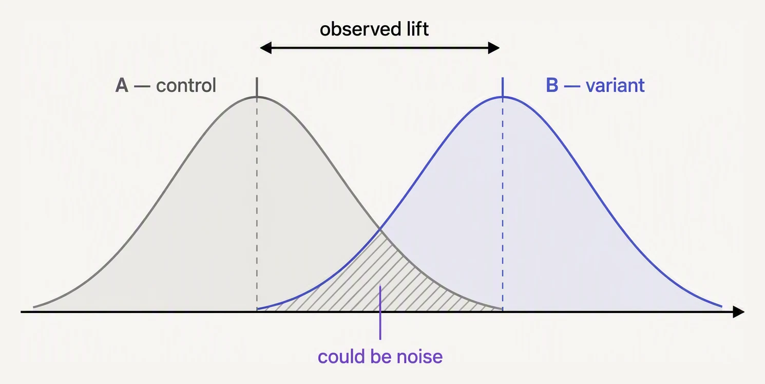
The question is never “is B bigger?” but “bigger than the noise?”
Two conversion rates: p_A (control) and p_B (treatment). The hypotheses are the familiar pair:
H0  (null):         p_A = p_B            "no real difference"
H1  (alternative):  p_A ≠ p_B            "there is a difference"
Then the test asks: if H0 were true, how surprising is the difference we actually saw? The answer
is the p-value — how often pure chance would produce a gap at least this large when H0 holds.
Surprising enough (p < 0.05 by convention), and you reject H0.
The object that makes “how often by chance” computable is the null distribution: the distribution of the observed difference assuming H0 is true. And here the CLT pays off exactly as promised. That difference of two proportions is approximately normal, centred at 0, with a standard error we can write down. Every number below flows from that one fact.
The two-proportion z-test
The standard test for comparing two conversion rates is five lines of arithmetic:
1. Compute observed rates:    p_A_hat,  p_B_hat
2. Compute pooled rate:       p_hat = (clicks_A + clicks_B) / (n_A + n_B)
3. Standard error:            SE = sqrt( p_hat (1-p_hat) (1/n_A + 1/n_B) )
4. Z-statistic:                z = (p_B_hat - p_A_hat) / SE
5. p-value (two-sided):        p = 2 * (1 - Φ(|z|))     Φ is normal CDF
Let’s run it on a concrete case: 5.2% versus 5.8% conversion, with 10,000 users per arm.
import numpy as np

from scipy.stats import norm

# Observed counts: 5.2% vs 5.8% conversion, n=10000 each
n_A, n_B = 10_000, 10_000
clicks_A = int(round(0.052 * n_A))   # 520
clicks_B = int(round(0.058 * n_B))   # 580

p_A_hat = clicks_A / n_A
p_B_hat = clicks_B / n_B
diff = p_B_hat - p_A_hat

# Pooled standard error
p_pool = (clicks_A + clicks_B) / (n_A + n_B)
se = np.sqrt(p_pool * (1 - p_pool) * (1/n_A + 1/n_B))

z = diff / se
p_value = 2 * (1 - norm.cdf(abs(z)))

print(f"p_A = {p_A_hat:.4f}, p_B = {p_B_hat:.4f}, lift = {diff:.4f}")
print(f"pooled p = {p_pool:.4f}, SE = {se:.5f}")
print(f"z = {z:.3f}")
print(f"p-value = {p_value:.4f}")
print("Significant at α=0.05?" , "yes" if p_value < 0.05 else "no")
p_A = 0.0520, p_B = 0.0580, lift = 0.0060
pooled p = 0.0550, SE = 0.00322
z = 1.861
p-value = 0.0627
Significant at α=0.05? noThe p-value lands at 0.063 — just over the line, not significant.
And this is the trap a great many teams fall straight into. The lift looks like a healthy 0.6 percentage points, an obvious win to the naked eye. Yet 10,000 per arm is not enough data to rule out chance at the 5% level. A meaningful-looking number and a statistically-powered number are different things.
Feel the boundary yourself — nudge the rates and sample sizes and watch the verdict flip:
Simulate an A/B test — then run it 100 times
Sample size: how big does each arm need to be?
The fix for a borderline result is not to stare harder. It is to have planned the sample size before launch, around the minimum detectable effect (MDE), the smallest lift you’d actually care about.
The standard formula for a two-proportion test at 80% power and α = 0.05:
n ≈ ( z_{α/2} + z_{β} )² · (p_A (1-p_A) + p_B (1-p_B)) / (p_B - p_A)²with z_{α/2} = 1.96 (two-sided α = 0.05) and z_{β} = 0.84 (80% power).
import numpy as np

from scipy.stats import norm

def sample_size(p_A, p_B, alpha=0.05, power=0.80):
    z_alpha = norm.ppf(1 - alpha / 2)
    z_beta  = norm.ppf(power)
    var_sum = p_A * (1 - p_A) + p_B * (1 - p_B)
    n = ((z_alpha + z_beta) ** 2 * var_sum) / (p_B - p_A) ** 2
    return int(np.ceil(n))

# How big does each arm need to be to detect a 0.6 percentage point lift on a 5.2% base?
n_needed = sample_size(p_A=0.052, p_B=0.058)
print(f"Sample size per arm for 5.2% → 5.8%: {n_needed:,}")

# What if you want to detect a 1.0 percentage point lift?
print(f"For 5.2% → 6.2%:                    {sample_size(0.052, 0.062):,}")

# What if you want to detect just 0.3 percentage points?
print(f"For 5.2% → 5.5%:                    {sample_size(0.052, 0.055):,}")
Sample size per arm for 5.2% → 5.8%: 22,660
For 5.2% → 6.2%: 8,434
For 5.2% → 5.5%: 88,319There is the lesson in three numbers. The 0.6-point lift we tested earlier actually needs ~22,700 per arm to detect reliably. That is more than double the 10,000 we used, which is why it came out borderline.
A generous 1.0-point lift needs only ~8,400. But a subtle 0.3-point lift demands ~88,000.
Halving the effect you want to catch roughly quadruples the sample. That is the 1/MDE² sitting
in the denominator, and it is the single most expensive fact in experimentation.
The pitfalls — what kills real A/B tests
1. Peeking
You check the p-value every day and stop “the moment it’s significant.” This inflates your false-positive rate badly. Randomness alone guarantees the p-value will dip below 0.05 at some point if you keep looking, even when H0 is perfectly true.
Here is an A/A test (no real difference at all) where the experimenter peeks every 1,000 users and
stops early on any p < 0.05:
# Simulation: run thousands of A/A tests (no real difference) where
# the experimenter "peeks" every 1000 users and stops if p<0.05.
import numpy as np

from scipy.stats import norm

rng = np.random.default_rng(0)
p_true = 0.05
n_max = 20_000
check_every = 1000
n_sim = 1000

false_positives = 0
for _ in range(n_sim):
    A = rng.binomial(1, p_true, size=n_max)
    B = rng.binomial(1, p_true, size=n_max)
    rejected = False
    for n_so_far in range(check_every, n_max + 1, check_every):
        a, b = A[:n_so_far].sum(), B[:n_so_far].sum()
        p_pool = (a + b) / (2 * n_so_far)
        se = np.sqrt(p_pool * (1 - p_pool) * (2 / n_so_far))
        if se == 0: continue
        z = (b - a) / (n_so_far * se)
        if 2 * (1 - norm.cdf(abs(z))) < 0.05:
            rejected = True
            break
    if rejected:
        false_positives += 1

print(f"False positive rate from peeking: {false_positives/n_sim:.2%}")
print("(Expected at α=0.05 if doing one final check: 5%)")
False positive rate from peeking: 22.40%
(Expected at α=0.05 if doing one final check: 5%)The nominal α was 5%; peeking 20 times blew the real false-positive rate to 22.4% — more than four times the rate you signed up for. Roughly one peeked “win” in five is pure illusion.
Sequential methods (mSPRT, alpha-spending) exist to license repeated looks honestly. But the simple discipline is: fix your sample size in advance and don’t look until you reach it.
2. Multiple comparisons
Testing 20 variants or 20 metrics? Even with no real effect, you’d expect one to cross p < 0.05 by
chance (5% × 20 ≈ 1 spurious winner). Correct the threshold (Bonferroni: divide α by the number of
tests) or control the false-discovery rate (Benjamini–Hochberg). The more hypotheses you fish
through, the higher your bar must climb.
3. Novelty effects
Users behave oddly in the first days of any visible UI change just because it is new. The lift you measure early may shrink — or reverse — once the novelty wears off. Run long enough to span multiple visit cycles: typically 1–2 weeks minimum, longer for low-frequency products.
4. Power for the wrong outcome
You powered the test for conversion lift, but the thing you truly care about is long-term revenue. Conversion can rise while revenue per user stays flat or falls. Decide your success metric before launch and size the experiment around that metric, not a convenient proxy.
In one breath
A/B testing pits H0: p_A = p_B against H1: p_A ≠ p_B. It asks how surprising the observed lift
would be under H0.
The null distribution of the difference is normal by the CLT. The
two-proportion z-test — pool the rate, form SE = √(p(1−p)(1/n_A+1/n_B)), compute
z = lift/SE, read p = 2(1−Φ(|z|)) — gives the p-value. Our 5.2% vs 5.8% at n = 10k landed at
0.063, not significant.
Plan with the sample-size formula: detecting half the effect costs 4× the data
(1/MDE²). So a 0.6-point lift needs ~22,700 per arm and a 0.3-point lift ~88,000.
Then dodge the four killers:
- peeking (here it quadrupled the false-positive rate to 22%);
- multiple comparisons;
- novelty; and
- powering for the wrong metric.
The math automates; the judgment does not.
Practice
Quick check
A question to carry forward
Look back at every formula in this lesson and notice the quiet move we never justified.
We wrote p_A_hat = clicks_A / n_A and treated it as the estimate of the true rate — obvious,
unarguable. Estimation did the same with the sample mean.
These all begin by plugging in “the” sample statistic as if no other choice existed:
- the z-test
- the t-test
- the confidence interval
But why is the sample proportion the right estimate of p? Why divide by n and not something
else? Some principle must be choosing these estimators — we have just never named it.
So here is the thread onward. Given data and a model with unknown parameters, what principle picks the single best parameter value — the one that makes the data you actually observed as likely as possible?
That is Maximum Likelihood Estimation (MLE), and the humble sample mean and sample proportion we have leaned on for five lessons will turn out to be its answers. The next questions are:
- What is a likelihood?
- Why does maximising it recover exactly these estimators?
- What does its Bayesian cousin MAP add when you also hold a prior belief?
Practice this in an interview
All questionsSample size, power, and MDE form a three-way trade-off: fix any two and the third is determined. You choose the MDE based on business materiality, then solve for the sample size that delivers 80–90 % power at alpha = 0.05.
The primary metric should be the closest measurable proxy for the user or business outcome you are trying to move, sensitive enough to detect a real change within your traffic budget. Guardrail metrics are the constraints — things that must not degrade even if the primary metric improves.
CUPED (Controlled-experiment Using Pre-Experiment Data) removes variance in the outcome metric that is explained by a pre-experiment covariate — typically the same metric measured before the experiment. This makes the residual variance smaller, which is equivalent to running a more powerful test or reaching significance faster with the same sample.
Run until you have reached the pre-calculated sample size — which should include at least one full weekly cycle to average out day-of-week effects. Stopping early because results look good, or extending because they do not, both inflate error rates.
A rigorous A/B test starts with a pre-registered decision, hypothesis, primary metric, randomization unit, minimum detectable effect, significance level, power, and fixed runtime. Random assignment, validated instrumentation, and a fixed analysis plan then estimate whether the change creates a practically worthwhile effect rather than a post-hoc false positive.
A non-significant result does not mean the treatment has no effect; it means the data are insufficient to distinguish the observed difference from noise at the specified power level. The correct interpretation depends entirely on the statistical power of the test — a well-powered flat result is evidence of no meaningful effect; an underpowered flat result is inconclusive.
Running many hypothesis tests simultaneously inflates the probability of at least one false positive far above the nominal alpha. Bonferroni correction addresses this by dividing alpha by the number of tests, guaranteeing the family-wise error rate stays at or below alpha — at the cost of reduced power per test.
Standard A/B tests assume the Stable Unit Treatment Value Assumption (SUTVA): one user's outcome is unaffected by another user's assignment. Network products violate this — a user in the control group can be affected by their friends in the treatment group, making naive estimates biased.
Novelty effect is the temporary engagement spike users show with any change simply because it is new; primacy effect is the temporary dip when users resist a change to a familiar interface. Both cause the short-term treatment effect to differ materially from the long-term steady-state effect.
P-hacking is the practice of making analytic choices — selecting metrics, segments, or time windows — after seeing data, guided by which choices produce p < 0.05. Multiple testing means that even without intent, testing many hypotheses at alpha = 0.05 expects one false positive per 20 tests.
A p-value measures the probability of seeing data at least as extreme as observed under the null hypothesis — it quantifies evidence against the null, not the magnitude of an effect. Effect size quantifies how large the difference or relationship is in meaningful units. With a large enough sample, a trivially small effect can produce an arbitrarily small p-value.
Peeking means checking statistical significance repeatedly during a test and stopping as soon as p drops below 0.05. Because the p-value fluctuates over time, this inflates the false-positive rate well above the nominal alpha — sometimes to 25–30 % for daily checks over a two-week test.
When randomization is not feasible — due to ethical, operational, or technical constraints — quasi-experimental designs such as difference-in-differences, regression discontinuity, and synthetic control can recover causal estimates, but each requires strong and testable assumptions.
Simpson's paradox occurs when a trend present in every subgroup reverses or disappears in the aggregate, because the subgroup sizes differ between treatment and control. In A/B tests it most often appears when the randomization is imbalanced across a strong confounding variable.
Bootstrapping estimates the sampling distribution of a statistic by repeatedly drawing samples with replacement from the observed data and computing the statistic on each resample. It works when the analytic sampling distribution is unknown, intractable, or the sample size is too small for asymptotic approximations to hold.