Why time series is different
Why you cannot treat time-stamped data like an ordinary tabular dataset — and what that forces you to do differently.
What you'll learn
- i.i.d. assumption: why ordinary ML relies on it and why time series breaks it
- Autocorrelation and ordering: the two structural facts that change everything
- Correct train/test splitting for time series: always keep the test set strictly in the future
Before you start
The visualization section closed on a quiet assumption hiding under almost every chart: that the rows were interchangeable — shuffle them and nothing is lost. This whole section is about the data where that assumption is exactly backwards, where the order of the rows is the entire point. Get this wrong and your model will look brilliant in testing and fail the moment it meets the future.
Ordinary ML assumes rows are i.i.d.
Every standard algorithm — logistic regression, random forests, gradient boosting, neural networks — is built on one quiet assumption: that your rows are i.i.d. (independent and identically distributed). Independent means knowing row 42 tells you nothing about row 43. Identically distributed means every row is drawn from the same underlying process.
When that assumption holds, you can shuffle your data, split it however you like, and a randomly chosen 20 % test set is a fair sample of the whole population. The ordering of rows is irrelevant noise.
Time series data breaks both parts of that assumption, always.
What makes time series structurally different
1. Observations are ordered
A row recorded on Monday is followed by Tuesday, then Wednesday. That order is not an accident — it is the data. Strip the order and you lose the thing you are trying to model.
2. Observations are correlated with their own past
Today’s sales depend on yesterday’s sales. Today’s temperature is closer to yesterday’s than to a random day six months ago. This self-correlation is called autocorrelation (the correlation of a series with a lagged copy of itself). It is not a nuisance to remove — it is the primary signal you are trying to exploit.
Because of autocorrelation, rows are not independent. Shuffle them and you destroy the very structure that makes prediction possible.
3. The data-generating process can drift
Related to autocorrelation is stationarity — whether the statistical properties (mean, variance) of the series change over time. You will explore this deeply in a later lesson. For now, just note that sales in December look nothing like sales in July; sensor readings drift as equipment ages. A random sample drawn from across the whole timeline may not represent the distribution your model will actually face at deployment.
The forecast horizon
When you build a time series model, you define a forecast horizon — how far ahead you want to predict. One day? One week? Three months? This matters because every evaluation protocol must respect it: the gap between the last training observation and the first test observation must be at least as large as the horizon you care about.
Typical domains where this matters:
- Retail demand — ordering inventory days or weeks ahead
- Energy prices — bidding in spot markets hours to days ahead
- IoT sensors — predictive maintenance before a failure occurs
- Web traffic — capacity planning for the next hour or day
In every case, at prediction time the future is genuinely unknown. Your evaluation must honour that.
The cardinal sin: shuffling time series data
The correct rule is simple: the test set must come strictly after the training set in calendar time. No exceptions.
Visualising correct vs wrong splits
The diagram below contrasts the correct forward-chaining split (top) with the wrong shuffled split (bottom).
Top: the test set is a clean future window. Bottom: shuffling scatters test rows across the full timeline, leaking future information into training.
Seeing structure that shuffling destroys
The code below synthesises a realistic-looking daily time series and then plots it alongside a version where the rows have been shuffled. The structure in the original — trend, rhythm, coherence — vanishes completely in the shuffled version. Any model trained on the shuffled version and tested on a random slice of it will absorb information from the future without knowing it.
import numpy as np
import matplotlib.pyplot as plt

np.random.seed(0)

days = np.arange(365)

trend     = 0.05 * days
seasonal  = 8 * np.sin(2 * np.pi * days / 7)
noise     = np.random.normal(0, 3, size=365)
series    = 100 + trend + seasonal + noise

shuffled  = series.copy()
np.random.shuffle(shuffled)

cutoff = 270

fig, axes = plt.subplots(2, 1, figsize=(10, 6), sharex=True)
fig.suptitle("365 days of synthetic sales data", fontsize=13, weight="bold")

axes[0].plot(days[:cutoff], series[:cutoff], color="#4f8ef7", lw=1.2, label="Train")
axes[0].plot(days[cutoff:], series[cutoff:], color="#f97316", lw=1.2, label="Test")
axes[0].axvline(cutoff, color="#888", lw=1, linestyle="--")
axes[0].set_title("Correct split — test is strictly in the future")
axes[0].set_ylabel("Sales")
axes[0].legend()

axes[1].plot(days[:cutoff], shuffled[:cutoff], color="#4f8ef7", lw=1.2, label="Train")
axes[1].plot(days[cutoff:], shuffled[cutoff:], color="#f97316", lw=1.2, label="Test")
axes[1].axvline(cutoff, color="#888", lw=1, linestyle="--")
axes[1].set_title("Wrong split — data shuffled before splitting")
axes[1].set_xlabel("Day")
axes[1].set_ylabel("Sales")
axes[1].legend()

plt.tight_layout()
plt.show()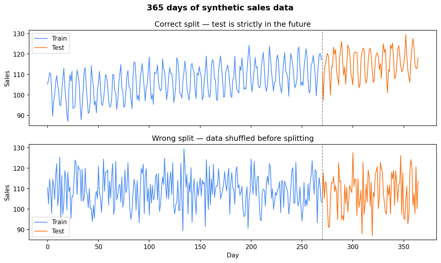
Top: ordered data drifts upward (~105→~118) with a weekly rhythm a model can learn. Bottom: shuffle the rows and the signal is gone — pure noise.
In the top panel you see an upward drift with a repeating weekly rhythm — the kind of pattern a forecasting model should learn (the level climbs from about 105 on day 1 to about 118 by day 365). In the bottom panel that structure is gone: the series looks like pure noise, because it is — the temporal order has been destroyed. The model trained on the bottom panel would learn nothing meaningful about how sales actually evolve.
What to do instead
For time series you have two correct evaluation strategies:
- Simple holdout — train on everything up to date T, test on everything after T. Fast and interpretable.
- Walk-forward (rolling) validation — repeatedly slide the training window forward, always predicting one step ahead into an unseen future. More robust, especially for shorter series.
You will implement both in the dedicated lesson on time series cross-validation.
Key vocabulary in one place
| Term | One-sentence definition |
|---|---|
| i.i.d. | Rows are drawn independently from the same distribution — standard ML assumption |
| Autocorrelation | The correlation of a series with a past (lagged) version of itself |
| Forecast horizon | How many steps into the future you need to predict |
| Data leakage | Training data that contains information about the future, inflating apparent performance |
| Stationarity | Whether the series’ statistical properties stay constant over time (preview for next lesson) |
In one breath
Ordinary ML assumes rows are i.i.d. — independent and identically distributed — so you can shuffle and a random test set is fair. Time series breaks that, always: observations are ordered (the order is the data), autocorrelated (today depends on yesterday — the signal you’re exploiting, not noise to remove), and drawn from a process that can drift (non-stationary). The cardinal sin is shuffling before splitting or using random K-fold: future rows leak into training, scores look great, production fails. The one rule that fixes it: the test set must come strictly after the training set in calendar time — a simple forward holdout, or walk-forward validation that slides the window forward and always predicts an unseen future.
Practice
Quick check
A question to carry forward
Look again at how we built that synthetic series: trend + seasonal + noise. We didn’t generate a
formless squiggle — we stacked a slow upward drift, a repeating 7-day wave, and random scatter, and the
sum looked convincingly like real sales. That’s not a coincidence of the demo; it’s how almost every
real-world series is structured.
So the question to carry forward is: if a time series is made of those parts, can you run the recipe in reverse — take a real series and pull the trend, the seasonality, and the noise back out as separate pieces you can inspect? That’s the first analytical move in all of time series. The next lesson, trend, seasonality and decomposition, does exactly that: it splits a real series into its components so you can see the growth without the weekly wiggle, the seasonal pattern on its own, and what’s left over — the part a model still has to explain.
Practice this in an interview
All questionsLag features shift the target or exogenous variables backward by k steps so the model sees past values as inputs; rolling features (rolling mean, std, min, max) summarise a window of past observations. Both must be computed strictly on past data — any feature that incorporates information from the current or future rows leaks the target and inflates metrics.
Walk-forward validation (also called time-series cross-validation or expanding-window CV) creates successive train/test folds where each fold's test set is always strictly in the future relative to its training set. It mimics real deployment — you fit on what you knew then and evaluate on what happened next — unlike random k-fold, which lets future data contaminate training.
Shuffling destroys temporal order, so the model trains on future data and is evaluated on the past — a direct information leak. Time series observations are serially correlated, meaning past values predict future ones, and any random split obliterates that structure entirely.
Standard k-fold randomly shuffles data, so a validation fold can contain timestamps earlier than the training fold — training on the future to predict the past. Time-series CV uses walk-forward (expanding-window or sliding-window) splits that always validate on data strictly after the training window.