VAR (multivariate)
Model several interdependent time series at once — interest rates, inflation, and unemployment — so that every variable's forecast draws on the past of every other variable in the system.
What you'll learn
- Vector AutoRegression: each series is regressed on its own lags AND the lags of every other series in the system
- Lag-order selection with AIC/BIC, and why all series must be stationary before fitting
- Granger causality and impulse response functions: testing and visualising cross-variable effects
Before you start
SARIMAX let an external driver push the target, but only one way — sales never pushed back on the holiday. The last lesson ended on the cases that break that assumption: series that are each both cause and effect. This lesson is the model for exactly that — no “driver” and “target,” just a system where every variable’s future leans on the recent past of every other.
Why separate ARIMAs are not enough
Suppose you fit an ARIMA on the unemployment rate using only its own past values. That model is blind to last quarter’s inflation reading, even if that reading reliably predicts where unemployment is heading. You lose signal every single period.
Vector AutoRegression (VAR) solves this by treating all K series as a joint system. At each time step, every variable is explained by p lags of itself and p lags of every other variable. The word vector signals that the outcome is not a scalar — it is the full column of values at time t.
The VAR(p) model
For a system with K variables and lag order p, the model at time t is:
y_t = c + A_1 y_{t-1} + A_2 y_{t-2} + ... + A_p y_{t-p} + e_twhere y_t is a column vector of length K (e.g. [interest_rate, inflation, unemployment]), each A_i is a K x K matrix of coefficients, c is a constant vector, and e_t is a vector of white-noise errors. The key insight is in the matrices: the off-diagonal entries let inflation’s past feed into the interest-rate equation, and vice versa. A separate ARIMA forces every off-diagonal to zero.
How many parameters are involved?
Each of the p lag matrices holds K x K coefficients, giving p * K^2 slope parameters plus K intercepts. With K = 3 variables and p = 4 lags that is already 36 slope parameters. Parameter count grows quadratically in K — keep the system small.
Interaction diagram
Step 1: Make every series stationary
VAR, like ARIMA, assumes stationarity. If your series are trended or otherwise non-stationary, difference them before fitting. You can run an Augmented Dickey-Fuller test on each column independently, then difference as needed.
Step 2: Choose the lag order p
You do not need to guess p. Fit models at several candidate orders and compare AIC (Akaike Information Criterion) or BIC (Bayesian Information Criterion). BIC penalises complexity more heavily and tends to favour parsimonious models, which is usually preferable when K is not tiny.
statsmodels can scan candidates automatically when you pass maxlags to .fit().
Step 3: Fit and forecast
import pandas as pd
from statsmodels.tsa.vector_ar.var_model import VAR

df = pd.read_csv("macro.csv", index_col="date", parse_dates=True)
df_diff = df.diff().dropna()

model = VAR(df_diff)
result = model.fit(maxlags=8, ic="bic")

print(result.summary())

lag_order = result.k_ar
forecast_input = df_diff.values[-lag_order:]
forecast = result.forecast(y=forecast_input, steps=4)
forecast_df = pd.DataFrame(forecast, columns=df_diff.columns)
print(forecast_df)Granger causality
After fitting you can ask a formal question: does knowing the past of variable X make forecasts of variable Y significantly more accurate, beyond what Y’s own past already tells us? This is called Granger causality — named after Clive Granger who formalised it.
Granger causality is not philosophical causality. It is a predictive test: X Granger-causes Y if lagged X has statistically significant coefficients in the Y equation.
from statsmodels.tsa.stattools import grangercausalitytests

results = grangercausalitytests(df_diff[["unemployment", "inflation"]], maxlag=4)
A low p-value on the F-test at a given lag means the lagged series does add predictive power.
Impulse response functions
After a shock to one variable — say, a sudden spike in the interest rate — how do the other variables respond over the following quarters? Impulse response functions (IRFs) trace that ripple through the system period by period.
irf = result.irf(periods=12)
irf.plot(orth=False)
Here is a real IRF grid from a fitted two-variable VAR where x was deliberately built to lead y (x’s past feeds y’s equation, but not the reverse):
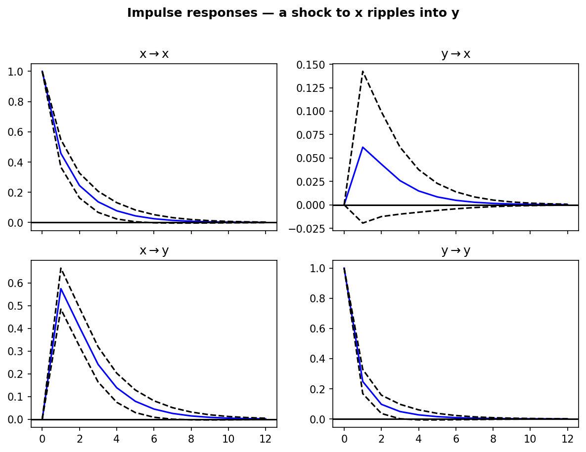
The bottom-left panel is the story: a shock to x ripples into y (peaks ~0.57, then fades). The top-right panel stays flat — y shocks don’t move x, exactly as the system was built.
IRFs are one of the most interpretable outputs of a VAR: each panel traces how a one-standard-deviation shock to one variable ripples through another over time. Read the bottom-left panel above and you can say “a shock to x lifts y for about five periods before it returns to baseline” — and read the flat top-right panel to confirm the influence runs one way, not both.
VAR versus separate ARIMAs — summary
| Property | Separate ARIMAs | VAR |
|---|---|---|
| Cross-variable effects | Ignored | Captured via off-diagonal lags |
| Parameters | K independent sets | p * K^2 shared slopes |
| Granger tests | Not possible | Built-in |
| Impulse responses | Not available | Available |
| Stationarity required | Per series | All series must be stationary |
In one breath
VAR(p) generalises AR from one series to a vector of K series: each variable is regressed on p lags
of itself and every other variable, y_t = c + A_1 y_(t-1) + … + A_p y_(t-p) + e_t, where the off-diagonal
entries of the K×K coefficient matrices are exactly the cross-variable links a separate ARIMA throws away.
The cost is quadratic — p·K² slopes — so keep the system small and pick p by AIC/BIC; and every series
must be stationary first (difference them) or the fit is spurious. Two payoffs only VAR gives you:
Granger causality (does X’s past add predictive power to Y beyond Y’s own past?) and impulse response
functions (trace how a shock to one variable ripples through the others over time).
Practice
Quick check
A question to carry forward
That closes the classical-models chapter — AR, MA, ARIMA, SARIMA, SARIMAX, VAR. Look back at what they all
demanded of you: test for stationarity, difference to the right order, squint at ACF and PACF to pick p
and q, fit, diagnose residuals, repeat. Powerful, but heavy — a lot of careful machinery per series.
So the question that opens the next chapter is a pragmatic one: is there a simpler, faster forecaster that just leans on recent data without all the diagnostics — one you could fit to thousands of series unattended? The next lesson, exponential smoothing and Holt-Winters, is that family (ETS): no stationarity tests, no order hunt — just a handful of smoothing knobs that weight recent observations more than old ones, often matching ARIMA on real data with a fraction of the fuss.
Practice this in an interview
All questionsA Vector Autoregression (VAR) model extends ARIMA to multiple time series simultaneously: each variable is regressed on its own past values and the past values of all other variables in the system. Use VAR when the series have mutual predictive relationships (Granger-causality) and you want to model those interactions; ARIMA is sufficient when one series can be forecast in isolation.
Prophet is a curve-fitting model that decomposes the series into trend, seasonality, and holidays; it handles missing data, multiple seasonalities, and non-uniform time grids with minimal tuning and is accessible to non-statisticians. ARIMA is a statistical model based on autocorrelation structure; it is more appropriate when the series is short, noise is small, and you need principled uncertainty intervals from an explicit stochastic process.
Multicollinearity occurs when two or more predictors are highly linearly correlated, inflating the variance of coefficient estimates and making them numerically unstable and uninterpretable. The Variance Inflation Factor (VIF) quantifies how much each coefficient's variance is inflated relative to an orthogonal design.
ARIMA(p,d,q) models non-seasonal series by combining autoregression, differencing, and a moving average of errors. SARIMA extends it with a second set of seasonal parameters (P,D,Q,s) that operate at the seasonal lag s, handling periodic patterns that ARIMA alone cannot capture.