Autoregression (AR)
Learn how the AR(p) model explains tomorrow as a weighted blend of recent history, and why the PACF tells you exactly how many lags to include.
What you'll learn
- AR(p) model: y_t as a linear combination of its own past p values plus white-noise error
- How phi controls persistence and mean-reversion in the AR(1) special case
- Why the PACF cuts off at lag p — the key diagnostic for choosing model order
Before you start
The last lesson read a fingerprint — “PACF cuts off after lag p → AR(p)” — while quietly leaning on a
process we never properly met: x_t = phi·x_{t-1} + noise. This lesson is the suspect behind that
fingerprint: what an AR model actually says, and why its PACF cuts off exactly where it does.
Why autoregression?
Many real-world time series carry momentum or persistence — a warm day tends to be followed by another warm day; a busy hour at a server often follows a busy hour. Autoregression (AR) is the workhorse model that captures exactly this structure. It forms the AR half of the famous ARIMA framework, so understanding it deeply pays dividends throughout forecasting work.
The core idea is disarmingly simple: treat the past values of the series itself as the predictors in an ordinary linear regression.
The AR(p) model
An AR(p) model says that the value at time t is a linear combination of its own p previous values plus a white-noise error term (a random shock with mean zero and constant variance):
y_t = c + phi_1·y_(t-1) + phi_2·y_(t-2) + ... + phi_p·y_(t-p) + e_t- c — a constant (the intercept, related to the series mean)
- phi_1 … phi_p — the autoregressive coefficients (the weights given to each lagged value)
- lag — a time-shifted copy of the series;
y_(t-1)is the series lagged by one period - e_t — white noise: independent, identically distributed errors with mean zero
- p — the order of the model, i.e. how many past values you look back
To fit an AR model you literally stack lagged columns of the series into a design matrix and run ordinary least squares. That is why the method is called autoregression — you regress the series on itself.
The AR(1) case in depth
The simplest non-trivial case, AR(1), uses only the immediately preceding value:
y_t = c + phi·y_(t-1) + e_tThe single coefficient phi controls everything interesting:
| phi value | Behaviour |
|---|---|
| phi close to +1 | Strong persistence — the series drifts slowly and stays near recent values for a long time |
| phi close to 0 | Weak memory — the series looks almost like random noise around its mean |
| phi negative | Mean reversion with oscillation — the series bounces above and below the mean each step |
Stationarity requirement: for the series to be stationary (have a stable, finite mean and variance), you need |phi| < 1. When |phi| = 1 you have a random walk; when |phi| > 1 the series explodes.
The PACF connection
In the previous lesson you learned that the Partial Autocorrelation Function (PACF) measures the correlation between y_t and y_(t-k) after removing the influence of all shorter lags. For a true AR(p) process, the PACF has a clean sharp cutoff after lag p — all partial autocorrelations beyond lag p are zero (within sampling noise). This is the primary diagnostic for choosing p: plot the PACF, find where it drops into the confidence band, and that lag is your order.
The AR feedback loop
The diagram below shows AR(1) as a feedback loop: the current output y_t is fed back as input y_(t-1) on the next step, scaled by phi, and combined with fresh noise e_t.
Simulate AR(1): see persistence change
The playground simulates two AR(1) series side by side — one with phi = 0.9 (high persistence) and one with phi = 0.3 (quick mean-reversion) — so you can see the difference directly.
import numpy as np
import matplotlib.pyplot as plt

np.random.seed(0)

def simulate_ar1(phi, n=200):
    y = np.zeros(n)
    for t in range(1, n):
        y[t] = phi * y[t-1] + np.random.normal(0, 1)
    return y

phi_high = 0.9
phi_low  = 0.3

y_high = simulate_ar1(phi_high)
y_low  = simulate_ar1(phi_low)

fig, axes = plt.subplots(2, 1, figsize=(8, 5), sharex=True)

axes[0].plot(y_high, color="#5b8dee", linewidth=1.0)
axes[0].axhline(0, color="#aaa", linewidth=0.6, linestyle="--")
axes[0].set_title(f"AR(1) with phi = {phi_high}  (high persistence)", fontsize=11)
axes[0].set_ylabel("y_t")

axes[1].plot(y_low, color="#e07b54", linewidth=1.0)
axes[1].axhline(0, color="#aaa", linewidth=0.6, linestyle="--")
axes[1].set_title(f"AR(1) with phi = {phi_low}  (quick mean-reversion)", fontsize=11)
axes[1].set_ylabel("y_t")
axes[1].set_xlabel("Time step")

plt.tight_layout()
plt.show()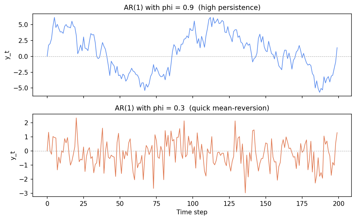
Same noise, two memories: phi = 0.9 (top) drifts in long runs; phi = 0.3 (bottom) snaps back to zero almost immediately.
What you see:
- The phi = 0.9 series drifts in long, sweeping runs — a positive excursion lasts many steps before the series returns to zero.
- The phi = 0.3 series bounces back toward zero rapidly; consecutive values look nearly independent.
- Both series are stationary because
|phi| < 1in both cases.
Editing phi to 0.99 makes the series look like a slow random walk; a negative value such as -0.7 gives the oscillating mean-reversion pattern.
Fitting AR with statsmodels
In practice you rarely simulate — you fit AR to observed data. The statsmodels library provides AutoReg. To prove it works, here we simulate an AR(2) with known coefficients (0.5 and 0.3) and check that the fit recovers them:
import numpy as np, pandas as pd
from statsmodels.tsa.ar_model import AutoReg

# Simulate AR(2): y_t = 0.5*y_{t-1} + 0.3*y_{t-2} + noise
np.random.seed(7)
N = 600
y = np.zeros(N)
for t in range(2, N):
    y[t] = 0.5 * y[t-1] + 0.3 * y[t-2] + np.random.normal(0, 1)
series = pd.Series(y)

result = AutoReg(series, lags=2).fit()   # AR(2)
print("params (const, phi_1, phi_2):", result.params.round(3).tolist())
print("forecast (5 steps):", result.forecast(steps=5).round(3).tolist())
params (const, phi_1, phi_2): [-0.063, 0.502, 0.274]
forecast (5 steps): [0.812, 0.643, 0.482, 0.355, 0.248]The fit recovers the true coefficients almost exactly — phi_1 = 0.502 (true 0.5) and phi_2 = 0.274 (true 0.3) — and the 5-step forecast decays smoothly back toward the series mean, exactly as an AR process should. On real data you’d skip the simulation and pass your own series; result.summary() reports the coefficients with standard errors, and AIC/BIC for comparing orders.
Choosing p in practice
- Plot the PACF of your (stationary) series. Count the lags before the bars drop inside the 95 % confidence band. That count is a good starting value for p.
- Information criteria (AIC, BIC) let you compare candidate orders rigorously —
AutoRegreports both. - Start small. AR(1) or AR(2) often captures most of the structure. Higher-order models may overfit.
In one breath
An AR(p) model predicts today as ordinary linear regression on its own last p values plus white noise:
y_t = c + phi_1·y_(t-1) + … + phi_p·y_(t-p) + e_t — you regress the series on itself. In the AR(1) case
the single phi controls memory: near +1 = long persistence (slow drifts), near 0 = rapid
mean-reversion (near-noise), negative = oscillating reversion — and stationarity demands |phi| < 1 (at
1 it’s a random walk, above it explodes). The PACF cuts off sharply at lag p, which is exactly how you
read the order off the plot before fitting; statsmodels.AutoReg then estimates the coefficients and
forecasts (recovering 0.5/0.3 from our simulated AR(2)). Start small — AR(1) or AR(2) captures most
structure; compare candidates with AIC/BIC.
Practice
Quick check
A question to carry forward
AR builds a forecast from past values — yesterday’s number, the day before’s. But look at where the
unpredictability actually enters: the e_t noise term, the shock at each step. AR treats those shocks
as throwaway once they’ve happened. Yet sometimes the lingering effect of a recent surprise — a stockout,
a viral post, a one-day outage — is the thing worth modelling, and an AR model captures it only awkwardly.
So the question to carry forward is: what if you built a model from the recent errors instead of the
recent values? The next lesson, moving average (MA), is exactly that complementary half of ARIMA —
y_t as a blend of the last few white-noise shocks — with the mirror-image fingerprint (ACF cuts off,
PACF tails off). Put AR and MA together and you have the full ARIMA engine.
Practice this in an interview
All questionsThe ACF measures correlation between a series and its own lags including indirect effects; the PACF strips out those indirect effects to show direct correlation at each lag. A cut-off in the PACF after lag p signals an AR(p) process; a cut-off in the ACF after lag q signals an MA(q) process.
A Vector Autoregression (VAR) model extends ARIMA to multiple time series simultaneously: each variable is regressed on its own past values and the past values of all other variables in the system. Use VAR when the series have mutual predictive relationships (Granger-causality) and you want to model those interactions; ARIMA is sufficient when one series can be forecast in isolation.
Choose d by differencing until the ADF test confirms stationarity; choose p from the PACF cutoff and q from the ACF cutoff on the differenced series; then confirm with AIC or BIC to guard against over-fitting. In practice, an automated grid search over a small range of candidates with information criteria is more reliable than visual inspection alone.
ARIMA(p,d,q) models non-seasonal series by combining autoregression, differencing, and a moving average of errors. SARIMA extends it with a second set of seasonal parameters (P,D,Q,s) that operate at the seasonal lag s, handling periodic patterns that ARIMA alone cannot capture.