Moving average (MA)
How MA(q) models the lingering effect of past shocks — and why it is nothing like a rolling-average smoother.
What you'll learn
- MA(q) formula: y_t equals the mean plus the current shock plus a weighted sum of the q previous shocks
- Why MA captures short-lived surprise effects while AR captures level persistence
- ACF cuts off at lag q — the signature diagnostic that identifies an MA process
Before you start
The last lesson ended on a hunch: AR builds forecasts from past values and throws the shocks away, but sometimes the lingering effect of a recent surprise is the thing worth modelling. This lesson is that idea made into a model — the complementary half of ARIMA, with the mirror-image fingerprint.
The MA(q) model in plain language
An autoregressive model says: today’s value is a weighted sum of recent past values plus noise. If sales were high yesterday they pull today’s sales up.
A moving-average model says something completely different: today’s value is the long-run mean plus a weighted sum of recent past surprises — not levels. A surprise, also called a shock or innovation, is the gap between what actually happened and what the model expected. Formally it is the white-noise error term, often written e_t (white noise means zero mean, constant variance, and no autocorrelation across time — each e_t is an independent draw from the same distribution).
The MA(q) model:
y_t = mu + e_t + theta_1 * e_(t-1) + theta_2 * e_(t-2) + ... + theta_q * e_(t-q)- mu is the unconditional mean of the series.
- e_t is the current shock (white noise, unknown until time t).
- e_(t-1) through e_(t-q) are the q most recent past shocks.
- theta_1 through theta_q are the MA coefficients (the weights on past shocks).
The order q is the “memory” of the model: how many past shocks still influence the present.
Why shocks, not levels?
Think of a central bank making an unexpected interest-rate announcement. That surprise ripples through markets for a day or two, then fades. The series does not stay permanently elevated — it absorbs the shock and returns to baseline. That is an MA signature: a short, sharp, finite-duration effect.
Compare that to AR, where a high value today raises the expected value tomorrow, which in turn raises the one after that, and so on. AR captures persistence in levels — effects can linger for many steps. MA captures persistence of surprises — effects are finite and die out after exactly q lags.
This distinction matters because the real world has both: a shock can push a series away from its mean (MA) while the series simultaneously tends to drift back toward it (AR). Combining them is exactly what ARIMA does.
The big naming confusion
How MA and AR look in a diagram
The diagram below contrasts the two feedback structures. In AR, past values of y loop back as inputs. In MA, past shocks (e) feed forward into the current value — there is no feedback from past y at all.
Top: MA(1) — only past shocks (e) feed into y_t; there is no recurrence on past y. Bottom: AR(1) shown for contrast — past values of y loop back. The two structures are genuinely different, not just reparameterisations.
The ACF signature: cuts off at lag q
Every model leaves a fingerprint in the autocorrelation function (ACF) — the correlation between y_t and y_(t-k) at various lags k.
For an MA(q) process the math works out cleanly: y_t shares error terms with y_(t-1) through y_(t-q) (they overlap in their shock windows), but y_t shares no error terms at all with y_(t-q-1) or anything earlier. That means:
- ACF is non-zero at lags 1 through q.
- ACF drops to (approximately) zero at lag q+1 and beyond.
This sharp cutoff is the fingerprint. If you plot an ACF and see significant bars only for the first q lags, suspect an MA(q) process.
Contrast with AR: AR’s PACF cuts off sharply at lag p, while its ACF decays gradually. MA and AR are mirror images in the ACF/PACF diagnostic table.
| ACF | PACF | |
|---|---|---|
| AR(p) | Decays gradually (tails off) | Cuts off after lag p |
| MA(q) | Cuts off after lag q | Decays gradually (tails off) |
| ARMA(p,q) | Tails off | Tails off |
Short memory is a feature, not a bug
An MA process has short memory by construction. No matter how large the theta coefficients are, the effect of any shock vanishes after exactly q steps. This makes MA models appropriate when shocks are transient — news events, measurement errors, one-off disruptions that are absorbed quickly.
AR models, by contrast, can have long memory depending on their coefficients: a near-unit-root AR(1) with phi close to 1 transmits shocks forward for many steps. Choosing between AR and MA (or combining them in ARMA/ARIMA) is largely a question of how fast the series recovers from a push.
Simulating and visualising MA(1)
The code below simulates 300 observations from an MA(1) process (y_t = e_t + 0.8 * e_(t-1)), plots the series, and shows the sample ACF so you can see the cutoff qualitatively.
import numpy as np
import matplotlib.pyplot as plt

np.random.seed(0)

n = 300
theta1 = 0.8
mu = 0.0

# Draw white-noise shocks
shocks = np.random.normal(0, 1, size=n + 1)

# Build MA(1): y_t = mu + e_t + theta1 * e_(t-1)
y = np.array([mu + shocks[t] + theta1 * shocks[t - 1] for t in range(1, n + 1)])

# --- manual ACF up to max_lag lags ---
max_lag = 20
acf_vals = []
y_centered = y - y.mean()
denom = np.sum(y_centered ** 2)
for k in range(max_lag + 1):
    if k == 0:
        acf_vals.append(1.0)
    else:
        numerator = np.sum(y_centered[k:] * y_centered[:-k])
        acf_vals.append(numerator / denom)

lags = np.arange(max_lag + 1)
conf = 1.96 / np.sqrt(n)   # approximate 95% confidence bound

fig, axes = plt.subplots(2, 1, figsize=(9, 6))

axes[0].plot(y, color="#4f8ef7", lw=0.9, alpha=0.85)
axes[0].axhline(mu, color="#f97316", lw=1.2, linestyle="--", label="mean (mu=0)")
axes[0].set_title("Simulated MA(1)  [theta_1 = 0.8, n=300]", fontsize=12)
axes[0].set_xlabel("Time step"); axes[0].set_ylabel("y_t"); axes[0].legend(frameon=False)

axes[1].bar(lags, acf_vals, color="#4f8ef7", alpha=0.75, width=0.6)
axes[1].axhline( conf, color="#f97316", lw=1.2, linestyle="--", label="95% confidence")
axes[1].axhline(-conf, color="#f97316", lw=1.2, linestyle="--")
axes[1].set_title("Sample ACF — expect significant bar at lag 1 only", fontsize=12)
axes[1].set_xlabel("Lag k"); axes[1].set_ylabel("Autocorrelation"); axes[1].set_xticks(lags); axes[1].legend(frameon=False)

plt.tight_layout()
plt.show()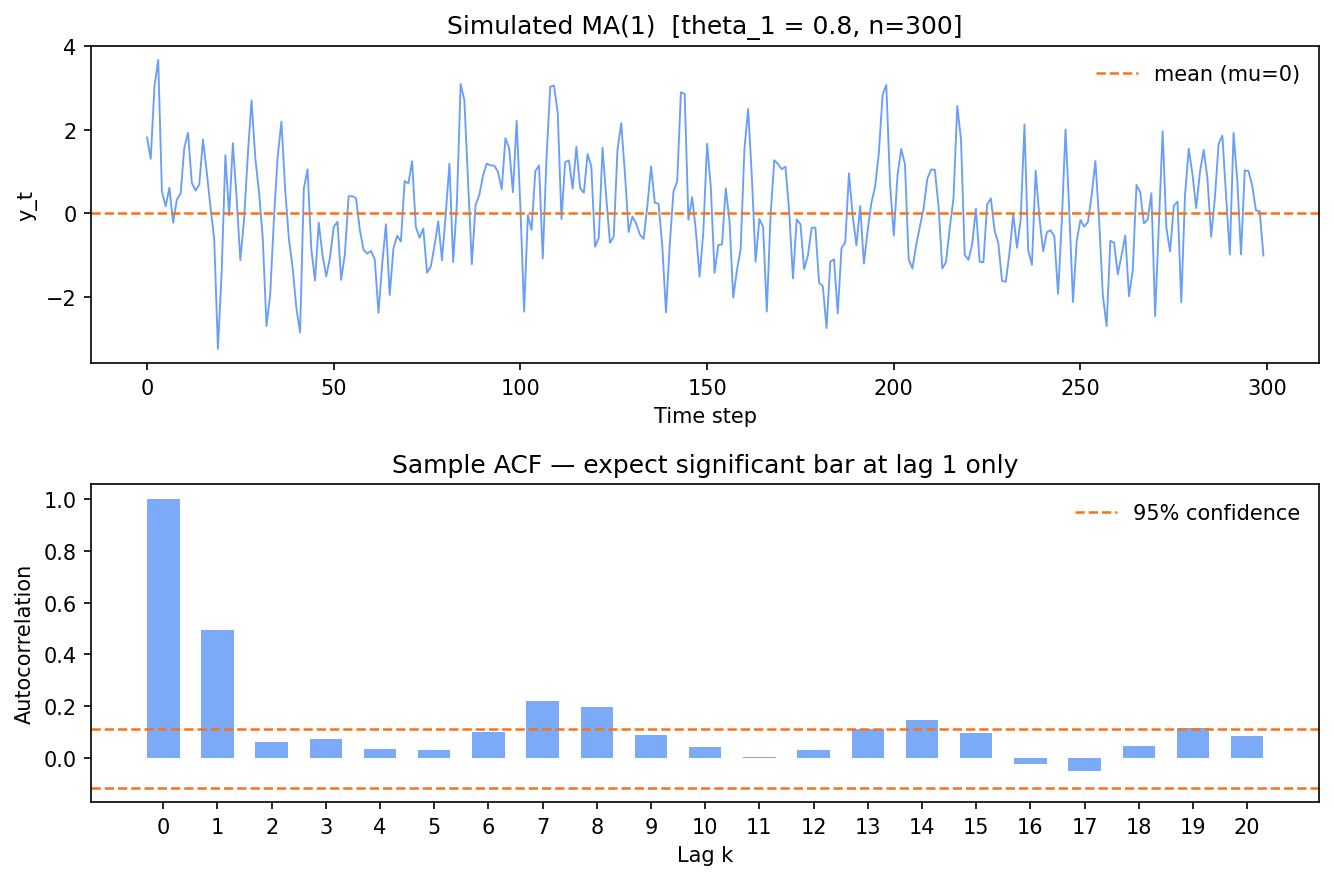
The MA(1) fingerprint: one significant ACF bar at lag 1 (≈0.49), then a sharp cutoff — every later lag is noise.
There’s the fingerprint: one prominent bar at lag 1 — measured ACF 0.49, matching the theoretical
theta / (1 + theta²) = 0.8/1.64 ≈ 0.488 — and the lag-2 bar already collapses to 0.06, inside the
confidence band. That sharp cutoff after lag 1 is the MA(1) signature. (Flip theta1 to -0.8 and the
lag-1 bar turns negative, but the cutoff pattern is unchanged.)
Fitting an MA model with statsmodels
The ARIMA class in statsmodels fits any combination of AR, differencing, and MA orders. To fit a pure MA(q) you set the AR order to 0 and the differencing order to 0. On the same simulated y (true theta = 0.8), the fit recovers it:
from statsmodels.tsa.arima.model import ARIMA

# Fit MA(1): order=(AR=0, I=0, MA=1)
result = ARIMA(y, order=(0, 0, 1)).fit()
print("Fitted theta_1:", round(result.params[result.param_names.index("ma.L1")], 3))
Fitted theta_1: 0.796The estimate 0.796 lands right on the true 0.8 — confirming both the model and the simulation. On real data you’d skip the simulation and pass your own series; result.summary() reports the coefficient with its standard error and the AIC/BIC for comparing orders.
MA in the context of ARIMA
ARIMA(p, d, q) combines three ideas:
- p — how many past values to include (AR part).
- d — how many times to difference to achieve stationarity (I part).
- q — how many past shocks to include (MA part).
A pure MA(q) is the special case ARIMA(0, 0, q). In practice, many real series need both AR and MA terms because levels persist (AR) and shocks reverberate for a few steps (MA). The combined model handles both at once, which is why ARIMA is the default workhorse for univariate time series forecasting.
In one breath
An MA(q) model builds today’s value from the long-run mean plus a weighted sum of the last q shocks
(white-noise surprises), not past values: y_t = mu + e_t + theta_1·e_(t-1) + … + theta_q·e_(t-q). Where
AR captures persistence in levels (effects linger geometrically), MA captures persistence of
surprises — a shock affects the series for exactly q steps then vanishes (short, finite memory). Its
fingerprint is the mirror image of AR: ACF cuts off after lag q while the PACF tails off. Beware the
name — this “moving average” is a model of the error process, not the rolling-window smoother (SMA)
that averages observed values. A pure MA(q) is just ARIMA(0, 0, q).
Practice
Quick check
A question to carry forward
You now hold both halves of the toolkit. AR models the persistence of levels; MA models the reverberation
of shocks; and a few lessons ago, differencing handled a drifting trend. We even kept naming the thing
that fuses them — every fit routine has been ARIMA(...), the AR and MA fingerprints share one diagnostic
table, and “a pure MA(q) is just ARIMA(0, 0, q).”
So the question to carry forward is the obvious one: how do the three ideas — autoregression, differencing, and moving average — combine into a single model you fit, diagnose, and forecast with? The next lesson, ARIMA(p, d, q), assembles them into the workhorse of univariate forecasting, walks the full Box-Jenkins workflow (stationarise → identify → fit → diagnose the residuals → forecast), and shows a real fit projecting forward with a confidence band that widens as the future gets hazier.
Practice this in an interview
All questionsMAPE (Mean Absolute Percentage Error) is intuitive and scale-free but breaks when actuals are near zero and penalises under-forecasts more than over-forecasts. MASE (Mean Absolute Scaled Error) solves both issues by scaling errors against a naive seasonal benchmark, making it valid even with zero values and comparable across series with different scales.
The ACF measures correlation between a series and its own lags including indirect effects; the PACF strips out those indirect effects to show direct correlation at each lag. A cut-off in the PACF after lag p signals an AR(p) process; a cut-off in the ACF after lag q signals an MA(q) process.
Regression to the mean is the statistical tendency for extreme measurements to be followed by measurements closer to the population mean, purely due to random noise — not because of any intervention. Analysts who intervene after observing an extreme value and then observe improvement often incorrectly attribute the recovery to their action.
Adam combines momentum (exponential moving average of gradients) with RMSProp-style adaptive per-parameter learning rates (exponential moving average of squared gradients). This means parameters with consistently large gradients get smaller effective steps, and sparse or small-gradient parameters get larger steps — making Adam nearly hyperparameter-free and fast-converging compared to vanilla SGD.