SARIMAX (exogenous regressors)
Add holiday flags, promo spend, price, and other known external drivers to a seasonal ARIMA model — and learn why forecasting with them requires knowing the future values of those drivers.
What you'll learn
- What the X in SARIMAX means: exogenous regressors are extra input columns, not lags of the target
- Model form: SARIMA captures autocorrelation in the residual after regressing on the exog variables
- Practical API: statsmodels SARIMAX, fitting with exog, and passing future exog to .forecast()
Before you start
The last lesson taught SARIMA every regular rhythm, but left it blind to irregular known events — a one-off promotion, a price cut, a drifting Easter. This lesson adds the final letter, X: a channel for handing the model exactly those external drivers, so they stop arriving as nasty surprises in the residuals.
The X in SARIMAX
SARIMAX is Seasonal AutoRegressive Integrated Moving Average with eXogenous regressors. Everything up to the X is the SARIMA you already know. The X adds one new idea:
An exogenous variable (from the Greek for “originating outside”) is a variable that influences your target series but is not itself predicted by the model. A holiday flag, promotional spend, a competitor’s price, or outdoor temperature are all exogenous to your sales. You observe or plan them ahead of time; they are inputs, not outputs.
Contrast this with the endogenous variable — the series you are trying to forecast (sales, in this example). The ARIMA terms model the endogenous variable’s own past. The exogenous terms model the additive lift or drag that each external driver provides on top of that.
How the model is structured
At its core SARIMAX combines two ideas in a single fit:
-
Regression on exog. Each exogenous column gets its own coefficient, exactly like ordinary linear regression. The model computes a weighted sum of the external signals and subtracts it from the target.
-
SARIMA on the residual. After removing the exog contribution, whatever is left is modelled with the full seasonal ARIMA structure: AR lags, differencing, MA error terms, and their seasonal counterparts at period s.
In words: the SARIMA part explains the autocorrelation that remains once the known external drivers are accounted for. The two pieces are estimated simultaneously in a single maximum-likelihood optimisation, so each part gets exactly the credit it deserves.
This means you can think of SARIMAX as answering two questions at once:
- How much does each external driver move the series? (regression coefficients)
- What pattern does the series follow on its own, after those drivers are removed? (SARIMA structure)
When exogenous regressors help
Adding exog variables is worthwhile when:
- You have known external drivers that repeat or can be planned (holidays, promotions, scheduled price changes, weather forecasts).
- Those drivers cause systematic deviations that your SARIMA residuals currently flag as unexplained spikes.
- You can supply future values of the drivers at forecast time — either because they are known (a public holiday calendar) or because you have a reliable separate forecast for them (a 7-day weather forecast).
Exog variables do not help when the driver is itself unpredictable, when you do not know its future value, or when its relationship with the target is highly nonlinear (in which case tree-based or neural models may be more appropriate).
The big trap: you must supply future exog
Diagram: external regressors feeding into the forecast
External regressors (holiday flag, promo spend) and the series’ own past both feed into SARIMAX. At forecast time the future rows of those regressors must be supplied.
Fitting SARIMAX in Python
The snippet below shows the complete workflow: build exogenous feature columns, fit the model, then pass the future rows of those same columns when forecasting.
import pandas as pd
from statsmodels.tsa.statespace.sarimax import SARIMAX

# --- Load target series and build exog columns ---
df = pd.read_csv("weekly_sales.csv", index_col="week", parse_dates=True)

# Exogenous feature matrix (aligned to the training index)
X_train = df[["is_holiday", "promo_spend"]]
y_train = df["sales"]

# --- Fit SARIMAX ---
# order=(p,d,q) for the non-seasonal part
# seasonal_order=(P,D,Q,s) for the seasonal part; here s=52 for weekly data
model = SARIMAX(
    y_train,
    exog=X_train,
    order=(1, 1, 1),
    seasonal_order=(1, 1, 1, 52),
    enforce_stationarity=False,
    enforce_invertibility=False,
)
result = model.fit(disp=False)
print(result.summary())

# --- Forecast the next 8 weeks ---
# You MUST provide X_future: 8 rows, same columns as X_train
X_future = pd.DataFrame({
    "is_holiday": [0, 0, 1, 0, 0, 0, 1, 0],   # two holidays in forecast window
    "promo_spend": [5000, 5000, 8000, 5000, 5000, 5000, 9000, 5000],
}, index=pd.date_range(df.index[-1], periods=8, freq="W"))

forecast = result.forecast(steps=8, exog=X_future)
print(forecast)To see that it actually works, here is a fit on a synthetic monthly series where every December gets a known +25 holiday lift. SARIMAX should recover that number:
# is_holiday is 1 every December, 0 otherwise; true lift built in = +25
result = SARIMAX(y, exog=X, order=(1,1,1), seasonal_order=(1,0,1,12),
                 enforce_stationarity=False, enforce_invertibility=False).fit(disp=False)
print("holiday coefficient:", round(result.params["is_holiday"], 2))
holiday coefficient: 27.04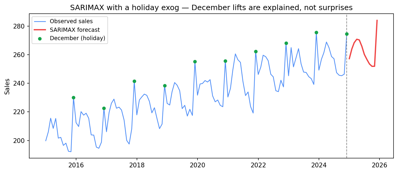
The fit recovers the holiday lift as 27.04 (true +25). The green December points are now explained by the exog coefficient, not left as surprise spikes in the residuals.
The estimate 27.04 lands close to the planted +25 — the model has learned the holiday effect as a single interpretable coefficient, and at forecast time it applies that same lift to the future Decembers you flag in X_future.
Reading the summary output
After fitting, result.summary() shows:
- Regression coefficients for each exog column (labelled by column name). A positive coefficient on
is_holidaymeans holidays lift sales on average; the magnitude is in the same units as your target. - AR, MA, seasonal AR, seasonal MA coefficients for the SARIMA part — these operate on the residual after the exog contribution is removed.
- AIC / BIC for model selection. Compare candidate orders by fitting multiple models and choosing the lowest AIC, holding the exog columns constant.
- Ljung-Box Q in the diagnostics — as always, the residuals should be white noise.
Diagnosing the model
result.plot_diagnostics(figsize=(12, 8))Inspect the residual ACF panel. If you still see systematic spikes — especially at the seasonal period — the SARIMA order needs adjusting. If you see a spike at lag 1 that disappears once you add the exog columns, the exog variables were absorbing autocorrelation that your SARIMA was missing, which is a sign they are genuinely helping.
Choosing your exogenous variables
Not every variable you might imagine deserves a slot in the exog matrix. A practical checklist:
- Is it known or forecastable ahead of time? A national holiday calendar is fixed years in advance. The spot price of a commodity might require a separate model to forecast, which introduces compounding error.
- Is its effect stable over time? If the relationship between promo spend and sales changes every year, a fixed linear coefficient will misfit.
- Does it reduce residual autocorrelation? Run the model with and without the candidate variable and compare the residual ACF and AIC. If neither improves, the variable is not adding useful signal beyond what the SARIMA terms already capture.
- Is it collinear with seasonal terms? A variable that fires every December is nearly collinear with the seasonal AR terms at s=12. The model will still fit, but the coefficients will be unstable and hard to interpret.
In one breath
SARIMAX = SARIMA + eXogenous regressors. The X is a set of external input columns — a holiday flag, promo spend, temperature, price — that drive the target but aren’t forecast from it (the endogenous series). Mechanically it’s two pieces fit together by one likelihood: a linear regression on the exog (each gets a coefficient), and SARIMA on whatever residual is left. So you learn both “how much each driver moves the series” and “the pattern it follows on its own.” The non-negotiable catch: to forecast h steps you must supply h rows of future exog, so only include drivers whose future you can actually obtain (a holiday calendar — yes; a competitor’s live price — risky). Confirm they help via AIC and a cleaner residual ACF, and beware exog that’s collinear with the seasonal terms.
Practice
Quick check
A question to carry forward
Notice the strict one-way street SARIMAX assumes: the exog drives the target, never the reverse. Holidays push sales; sales don’t push holidays. That’s why you can plan the future exog independently. But a huge class of problems breaks exactly that assumption. Ad-spend lifts sales — and a good sales quarter loosens next quarter’s ad budget. Two competing stocks tug on each other. Interest rates and inflation chase one another. Each series is both cause and effect.
So the question to carry forward is: how do you model several series that mutually influence one another, where there’s no clean split into “driver” and “target”? The next lesson, VAR (vector autoregression), generalises AR to a vector of series, letting every variable’s forecast depend on the recent past of all of them — the multivariate workhorse for genuinely interdependent time series.
Practice this in an interview
All questionsARIMA(p,d,q) models non-seasonal series by combining autoregression, differencing, and a moving average of errors. SARIMA extends it with a second set of seasonal parameters (P,D,Q,s) that operate at the seasonal lag s, handling periodic patterns that ARIMA alone cannot capture.
A Vector Autoregression (VAR) model extends ARIMA to multiple time series simultaneously: each variable is regressed on its own past values and the past values of all other variables in the system. Use VAR when the series have mutual predictive relationships (Granger-causality) and you want to model those interactions; ARIMA is sufficient when one series can be forecast in isolation.
Prophet is a curve-fitting model that decomposes the series into trend, seasonality, and holidays; it handles missing data, multiple seasonalities, and non-uniform time grids with minimal tuning and is accessible to non-statisticians. ARIMA is a statistical model based on autocorrelation structure; it is more appropriate when the series is short, noise is small, and you need principled uncertainty intervals from an explicit stochastic process.
Decomposition separates a series into a trend component (long-run direction), a seasonal component (periodic, fixed-period pattern), and a residual (everything left over). Additive decomposition sums the three; multiplicative decomposition multiplies them, which is appropriate when seasonal swings grow with the level.