Prophet
Learn how Meta's Prophet decomposes a time series into trend, seasonality, and holiday effects — and why its analyst-friendly API makes it a go-to for business forecasting.
What you'll learn
- Prophet's additive model: trend + seasonality + holidays + noise, fit by curve-fitting rather than Box-Jenkins
- Automatic changepoint detection: how Prophet finds trend shifts without manual parameter tuning
- The Prophet API: preparing a ds/y DataFrame, calling fit and predict, and adding holidays or regressors
Before you start
The last lesson made ETS light, but it still assumed a tidy world — one clean season, no gaps, no holidays. The mess that breaks it (two seasonalities at once, irregular holidays, missing days) is precisely what this model was built for: forecasting for people who don’t want to become time-series experts first.
Why Prophet exists
ARIMA is powerful, but it demands careful stationarity testing, ACF/PACF reading, and manual order selection. Scale that to dozens of series with business calendars and irregular gaps, and the workflow becomes expensive.
Prophet — released by Meta’s Core Data Science team in 2017 — was designed for exactly that situation. Its core insight is that most business time series are well described by a sum of interpretable components. Rather than modelling autocorrelation structure, Prophet fits a regression-style curve to each component separately. The result:
- Gaps and outliers affect the curve-fit much less than they affect ARIMA.
- Seasonality and holidays are first-class inputs, not afterthoughts.
- Non-statisticians can configure and inspect results without reading a textbook.
Prophet’s additive model
Prophet decomposes every forecast into four pieces:
y(t) = trend(t) + seasonality(t) + holidays(t) + noiseEach term is explained below. The diagram after this section shows how they combine visually.
Trend with automatic changepoints
A changepoint is a moment when the underlying growth rate shifts — a product launch, a policy change, a market shock. In Prophet the trend is piecewise-linear (or optionally piecewise-logistic for series with a natural ceiling). Prophet scans a set of candidate changepoint locations — by default the first 80 % of the training data — and uses a sparse prior to select only the ones actually supported by the data. You rarely need to specify them by hand.
from prophet import Prophet

m = Prophet()
You can override defaults:
m = Prophet(
    growth="logistic",          # use when the series has a known cap
    changepoint_prior_scale=0.05,  # lower = smoother trend
    n_changepoints=25,          # number of candidate changepoints
)
Seasonality via Fourier terms
Rather than dummy variables, Prophet models seasonality with Fourier series — sums of sine and cosine waves at the relevant period. Yearly seasonality uses 10 Fourier pairs by default; weekly uses 3. This makes the seasonal pattern smooth and continuous, which is realistic for most business phenomena. You can add custom seasonalities (monthly, quarterly) with a single method call.
Holiday effects
Holiday effects are short, sharp pulses — a sales spike on a public holiday, a traffic drop on a long weekend. Prophet lets you pass a DataFrame of known dates, and it estimates a separate coefficient for each holiday window. This is far more reliable than hoping the model learns it from data alone.
Noise
The residual noise term absorbs everything not explained by the three structured components. Prophet assumes it is white noise; if your residuals show remaining autocorrelation, that is a signal to add a custom seasonality or regressor.
The inline-SVG diagram
The Prophet API
Step 1 — Prepare the DataFrame
Prophet requires exactly two columns: ds (datestamp, as a pandas datetime) and y (the numeric target). Column names are mandatory; Prophet will raise an error if they are absent.
import pandas as pd
from prophet import Prophet

df = pd.read_csv("daily_sales.csv", parse_dates=["date"])
df = df.rename(columns={"date": "ds", "sales": "y"})
Missing rows are fine — Prophet interpolates across gaps during curve fitting.
Step 2 — Fit
m = Prophet(yearly_seasonality=True, weekly_seasonality=True)
m.fit(df)
Fitting calls Stan under the hood via L-BFGS (default) or MCMC for full uncertainty quantification.
Step 3 — Build the future DataFrame and predict
make_future_dataframe appends periods rows of future dates to the training dates. Calling predict returns a DataFrame with one row per date and columns including yhat (point forecast), yhat_lower, and yhat_upper (uncertainty intervals).
future = m.make_future_dataframe(periods=90, freq="D")
forecast = m.predict(future)

print(forecast[["ds", "yhat", "yhat_lower", "yhat_upper"]].tail())
Step 4 — Plot components
fig = m.plot_components(forecast)This renders separate panels for trend, weekly seasonality, yearly seasonality, and any holidays — which is where Prophet earns its “interpretable” reputation.
Adding holidays
Pass a DataFrame with columns holiday (name string) and ds (date). Prophet fits a separate coefficient for each named holiday.
from prophet.make_holidays import make_holidays_df

holidays = make_holidays_df(year_list=[2023, 2024, 2025], country="US")
m = Prophet(holidays=holidays)
m.fit(df)
For non-standard events (a product launch, a campaign start), add them to the same holidays DataFrame with a custom name.
Adding external regressors
A regressor is an additional time-varying input — a price index, a temperature reading, a promotional flag — that you believe drives y. Prophet treats it as another additive term.
m = Prophet()
m.add_regressor("promo_flag")
m.fit(df)   # df must also contain a column named promo_flag

future["promo_flag"] = 0   # fill in future values of the regressor
forecast = m.predict(future)
The regressor must be known for the forecast horizon, which is the main practical constraint.
Strengths and limits
Where Prophet shines
- Analyst-friendly: a non-statistician can configure seasonalities and holidays without touching ACF/PACF plots.
- Interpretable components: the components plot separates what is trend from what is seasonal, making results auditable.
- Robust to gaps and outliers: curve-fitting degrades gracefully; an ARIMA fit would fail or need imputation.
- Scales horizontally: the same API runs on hundreds of product lines with minimal per-series tuning.
Real limits
Putting it together: a minimal working example
import pandas as pd
from prophet import Prophet

df = pd.read_csv("daily_sales.csv", parse_dates=["date"])
df = df.rename(columns={"date": "ds", "sales": "y"})

m = Prophet(
    yearly_seasonality=True,
    weekly_seasonality=True,
    changepoint_prior_scale=0.05,
)
m.fit(df)

future = m.make_future_dataframe(periods=90, freq="D")
forecast = m.predict(future)

fig1 = m.plot(forecast)
fig2 = m.plot_components(forecast)
Run on a two-year daily series with weekly and yearly rhythms, m.plot(forecast) gives the fitted curve and a 90-day-ahead band:
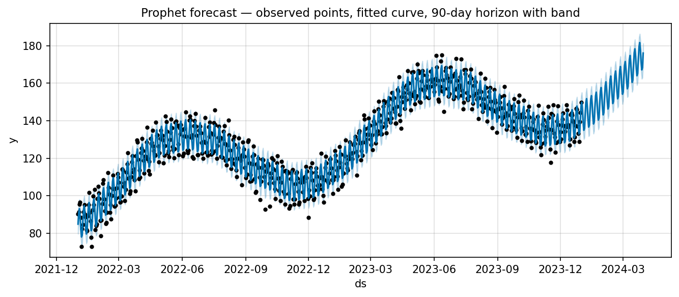
m.plot(forecast): observed points, fitted curve, and a 90-day-ahead forecast with its uncertainty band.
But the panel that earns Prophet its “interpretable” reputation is m.plot_components(forecast), which pulls the forecast apart into its additive pieces:
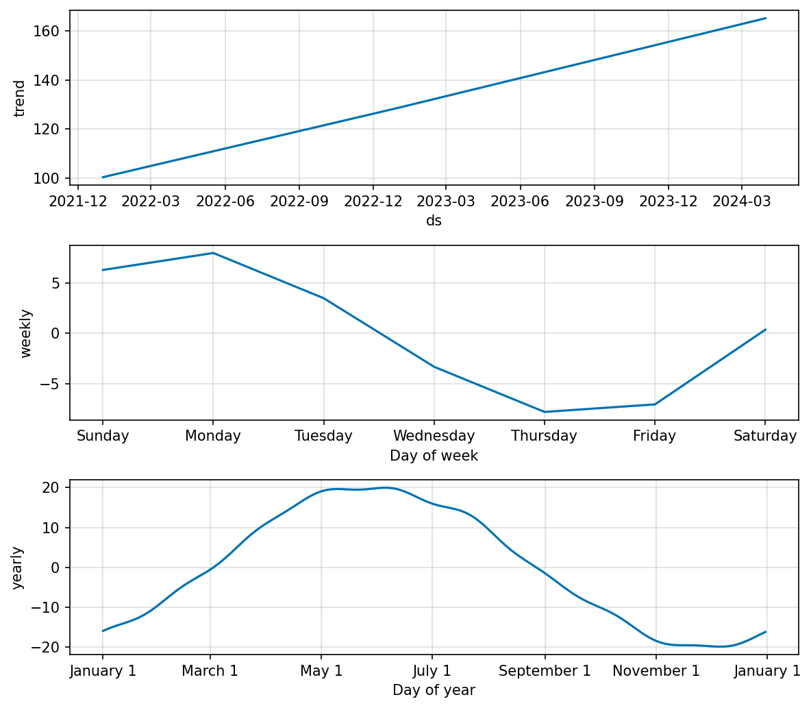
plot_components separates trend, weekly, and yearly seasonality — here recovering the Monday peak and the May high baked into the data. This is what “auditable” means.
Run this, look at the components plot, sanity-check the trend, then evaluate on a held-out window before calling the model production-ready.
In one breath
Prophet (Meta, 2017) trades Box-Jenkins for a decomposition fit: y(t) = trend + seasonality + holidays + noise, each piece a smooth curve rather than an autocorrelation structure. The trend is
piecewise-linear with automatic changepoints (it scans candidate dates and a sparsity prior keeps only
real shifts); seasonality is Fourier series (smooth sine/cosine waves, multiple periods at once);
holidays are known-date pulses you supply; regressors are extra additive inputs (whose future
values you must provide). The API is two columns — ds, y — then fit, make_future_dataframe,
predict, and the signature plot_components. It shines on messy business series (gaps, outliers, holidays,
many series at scale) and is analyst-friendly — but it’s not magic: changepoints can overfit recent noise,
so always inspect components and validate on a held-out window.
Practice
Quick check
A question to carry forward
Step back and notice what Prophet, ARIMA, SARIMA, and ETS all have in common: each is a specialized
time-series model, with its own assumptions and its own API. But there’s a whole world of general-purpose
models — XGBoost, LightGBM, random forests — that routinely win tabular-prediction competitions and that
none of these time-series tools let you use. They expect a plain (X, y) feature table with i.i.d. rows,
which is exactly what a raw time series is not.
So the question to carry forward is: can you reframe forecasting as ordinary supervised learning —
turn “predict the next value” into “predict y from a table of features derived from the past” — so any
regressor you like can do the job? The next lesson, lag and rolling features, is that bridge: how to
build lag columns, trailing-window statistics, and calendar features into a leakage-free feature table that
hands a time series to XGBoost or any tabular model.
Practice this in an interview
All questionsProphet is a curve-fitting model that decomposes the series into trend, seasonality, and holidays; it handles missing data, multiple seasonalities, and non-uniform time grids with minimal tuning and is accessible to non-statisticians. ARIMA is a statistical model based on autocorrelation structure; it is more appropriate when the series is short, noise is small, and you need principled uncertainty intervals from an explicit stochastic process.
Decomposition separates a series into a trend component (long-run direction), a seasonal component (periodic, fixed-period pattern), and a residual (everything left over). Additive decomposition sums the three; multiplicative decomposition multiplies them, which is appropriate when seasonal swings grow with the level.
Simple exponential smoothing computes a weighted average of all past observations where weights decay geometrically, controlled by a single smoothing parameter alpha. Holt's method adds a trend component with a second parameter beta; Holt-Winters (ETS) adds a seasonal component with a third parameter gamma, making it a strong baseline for series with both trend and seasonality.
MAPE (Mean Absolute Percentage Error) is intuitive and scale-free but breaks when actuals are near zero and penalises under-forecasts more than over-forecasts. MASE (Mean Absolute Scaled Error) solves both issues by scaling errors against a naive seasonal benchmark, making it valid even with zero values and comparable across series with different scales.