SARIMA (Seasonal ARIMA)
Extend ARIMA with a second set of seasonal AR, differencing, and MA terms that operate at lag m — the season length — so the model captures yearly, weekly, or any repeating cycle.
What you'll learn
- SARIMA(p,d,q)(P,D,Q)m: what each of the seven parameters controls and how the seasonal block differs from the ordinary block
- Seasonal differencing D: subtracting the value one full season ago to remove a periodic mean shift
- Reading ACF/PACF spikes at multiples of m to choose P and Q
Before you start
The last lesson ended on ARIMA’s blind spot: a stubborn spike at lag 12 (monthly) or lag 7 (daily) that
keeps reappearing in the residuals no matter how you tune p, d, q. That spike is the seasonal cycle
the model has no vocabulary for. SARIMA gives it that vocabulary — a second block of terms that operate
“versus last December,” not just “versus last month.”
Why ARIMA is not enough for seasonal data
ARIMA(p, d, q) models short-range autocorrelation (observations a few lags apart) and trend (via ordinary differencing). It knows nothing about observations separated by exactly one season — 12 months for monthly-yearly data, 7 days for daily-weekly data, 4 quarters for quarterly-yearly data.
If your series has a strong seasonal cycle, residuals from a plain ARIMA model will still carry spikes at multiples of the season length m. Those spikes mean signal the model has not absorbed. SARIMA absorbs them by adding a seasonal block of terms that work at lag m, 2m, 3m, and so on.
The SARIMA notation
SARIMA(p, d, q)(P, D, Q)m
The notation stacks two ARIMA-style triplets:
| Symbol | Block | Role |
|---|---|---|
| p, d, q | Ordinary (non-seasonal) | Short-range AR lags, trend differencing, short-range MA lags |
| P, D, Q | Seasonal | Seasonal AR lags at multiples of m, seasonal differencing, seasonal MA lags at multiples of m |
| m | Period | Number of time steps in one season (12 = monthly/yearly, 7 = daily/weekly, 4 = quarterly/yearly) |
The seasonal block mirrors the ordinary block exactly — it just stretches the lag axis by a factor of m. A seasonal AR term at order P = 1 uses the observation from m steps ago, not just one step ago.
Seasonal differencing D
Ordinary differencing (parameter d) subtracts the previous observation to remove a linear trend:
y't = yt - y(t-1)Seasonal differencing (parameter D) subtracts the observation exactly one full season ago to remove a repeating seasonal mean shift:
y't = yt - y(t-m)If your monthly sales always rise in summer and fall in winter, subtracting the value from the same month last year cancels that cycle. After D = 1 seasonal difference, the seasonal pattern is — in principle — gone, leaving only irregular variation that the AR and MA terms can model.
You can apply both ordinary and seasonal differencing together. d = 1, D = 1 means you first seasonally difference and then ordinary-difference the result (or vice versa). The total order of integration is d + D.
Identifying P and Q from the ACF and PACF
The same ACF/PACF logic that drives ordinary (p, q) selection applies to the seasonal block, but you read the plots at the seasonal lags m, 2m, 3m rather than lags 1, 2, 3.
- Spike in the PACF at lag m (and perhaps 2m), ACF decaying slowly at seasonal lags — suggests a seasonal AR term (P = 1 or 2).
- Spike in the ACF at lag m (and perhaps 2m), PACF decaying slowly at seasonal lags — suggests a seasonal MA term (Q = 1 or 2).
- Both decay gradually at seasonal lags — a mixed seasonal ARMA may help, though parsimony favors keeping P and Q small.
For the ordinary block you read the same plots at lags 1, 2, 3 as you would for a plain ARIMA.
The inline diagram
A seasonal series peaks at every multiple of m. The seasonal block (P, D, Q) models the autocorrelation at those lags; the ordinary block (p, d, q) handles everything in between.
Fitting with statsmodels
statsmodels exposes SARIMA through its SARIMAX class (the X stands for optional exogenous regressors; you can ignore it for pure SARIMA). The order argument takes the ordinary triplet and seasonal_order takes the seasonal triplet plus the period m.
import pandas as pd
from statsmodels.tsa.statespace.sarimax import SARIMAX

# monthly_sales is a pandas Series with a DatetimeIndex, freq="MS"
model = SARIMAX(
    monthly_sales,
    order=(1, 1, 1),           # p=1, d=1, q=1
    seasonal_order=(1, 1, 1, 12),  # P=1, D=1, Q=1, m=12
    enforce_stationarity=False,
    enforce_invertibility=False,
)
result = model.fit(disp=False)

print(result.summary())

# 12-step-ahead forecast
forecast = result.get_forecast(steps=12)
mean_forecast = forecast.predicted_mean
conf_int = forecast.conf_int()Run that on a synthetic monthly series with a clear yearly cycle and the payoff is visible at a glance — the forecast doesn’t flatten, it keeps cycling:
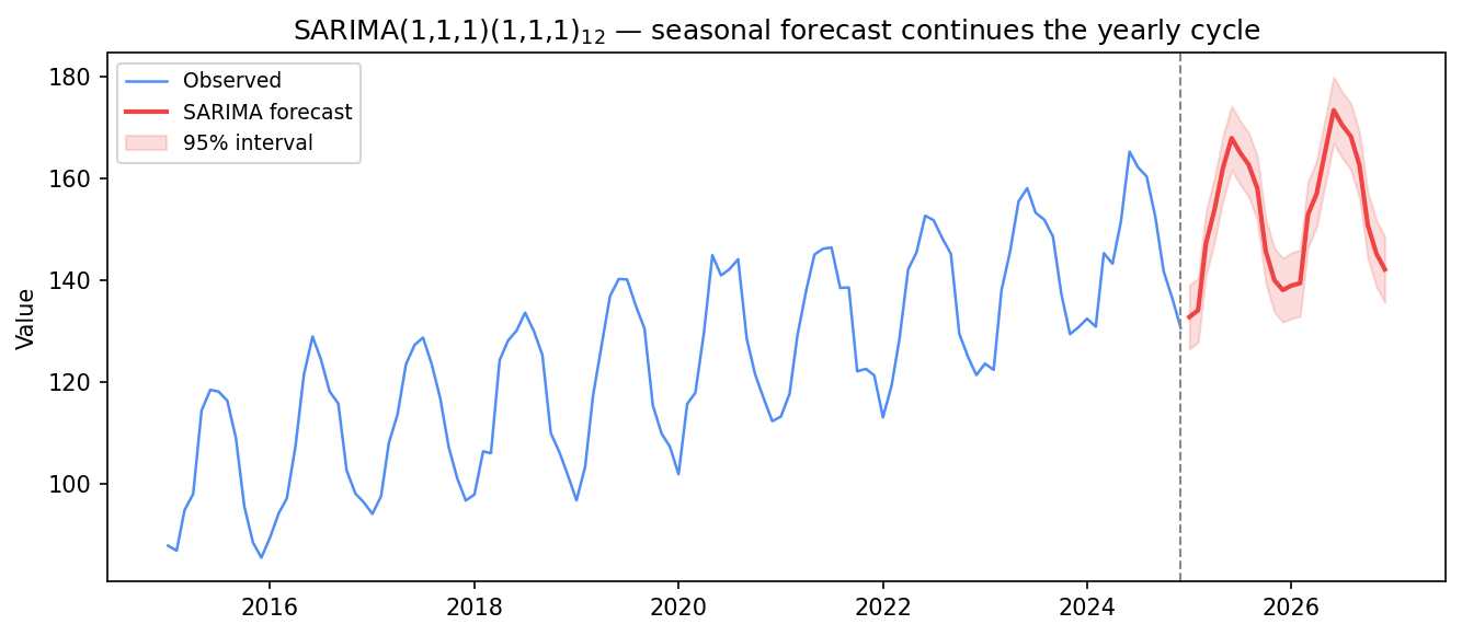
SARIMA(1,1,1)(1,1,1)12 (AIC 495.8): the forecast reproduces the yearly humps rather than flattening — exactly the cycle a plain ARIMA would miss.
That is the whole point of the seasonal block: where a non-seasonal ARIMA forecast decays to a flat level, SARIMA carries the repeating peaks and troughs forward into the future.
Reading the summary
The summary table from result.summary() lists coefficients for each AR, MA, seasonal AR, and seasonal MA term along with p-values. Coefficients that are not statistically significant (large p-values, typically above 0.05) suggest you may be over-parameterizing — try reducing P or Q by one. After fitting, inspect residuals with result.plot_diagnostics(): the residual ACF should show no spikes at any lag, including the seasonal ones.
Choosing m
m must match the true periodicity in your data. Common choices:
- m = 12 — monthly data with a yearly cycle
- m = 7 — daily data with a weekly cycle
- m = 4 — quarterly data with a yearly cycle
- m = 24 — hourly data with a daily cycle
If you are unsure of m, plot the raw series and look for the distance between recurring peaks. A seasonal decomposition (STL or classical) can also reveal the dominant period before you commit to a value.
SARIMA vs plain ARIMA — a summary
| Feature | ARIMA(p,d,q) | SARIMA(p,d,q)(P,D,Q)m |
|---|---|---|
| Handles trend | Yes (via d) | Yes (via d) |
| Handles seasonality | No | Yes (via D and seasonal terms) |
| ACF/PACF spikes at lag m | Left unmodeled | Absorbed by P or Q |
| Parameters to choose | 3 | 7 |
| Typical use | Non-seasonal or weakly seasonal | Monthly, daily, quarterly with clear cycle |
In one breath
SARIMA(p,d,q)(P,D,Q)m bolts a second, seasonal ARIMA block onto the ordinary one, operating
at the season length m (12 monthly, 7 daily, 4 quarterly). The seasonal block mirrors the ordinary one
but stretches the lag axis by m: seasonal differencing D subtracts the value one full season ago
(y_t − y_(t−m)) to kill a repeating mean shift, and seasonal AR/MA (P, Q) model the autocorrelation at
lags m, 2m, 3m — which you read off ACF/PACF at the seasonal lags, not lags 1, 2, 3. Usually d=1, D=1
suffices; don’t over-difference. Fit it via statsmodels’ SARIMAX (seasonal_order=(P,D,Q,m)), and the
forecast carries the cycle forward instead of flattening.
Practice
Quick check
A question to carry forward
SARIMA now captures any regular rhythm — the December peak, the Monday dip — because those repeat on a fixed clock. But notice what it still can’t see: the irregular events you nonetheless know are coming. A one-off Black Friday promotion. A price cut next month. An Easter that drifts across the calendar. These aren’t periodic, so no seasonal term will ever learn them — and SARIMA keeps getting “surprised” by things already on your calendar.
So the question to carry forward is: how do you hand the model external information it can’t infer from the series’ own past? The next lesson, SARIMAX, adds the X — exogenous regressors like a holiday flag or promo spend — so the model treats them as known drivers, with one crucial catch: to forecast with them, you must supply their future values too.
Practice this in an interview
All questionsARIMA(p,d,q) models non-seasonal series by combining autoregression, differencing, and a moving average of errors. SARIMA extends it with a second set of seasonal parameters (P,D,Q,s) that operate at the seasonal lag s, handling periodic patterns that ARIMA alone cannot capture.
A Vector Autoregression (VAR) model extends ARIMA to multiple time series simultaneously: each variable is regressed on its own past values and the past values of all other variables in the system. Use VAR when the series have mutual predictive relationships (Granger-causality) and you want to model those interactions; ARIMA is sufficient when one series can be forecast in isolation.
Prophet is a curve-fitting model that decomposes the series into trend, seasonality, and holidays; it handles missing data, multiple seasonalities, and non-uniform time grids with minimal tuning and is accessible to non-statisticians. ARIMA is a statistical model based on autocorrelation structure; it is more appropriate when the series is short, noise is small, and you need principled uncertainty intervals from an explicit stochastic process.
Choose d by differencing until the ADF test confirms stationarity; choose p from the PACF cutoff and q from the ACF cutoff on the differenced series; then confirm with AIC or BIC to guard against over-fitting. In practice, an automated grid search over a small range of candidates with information criteria is more reliable than visual inspection alone.