Trend, seasonality & decomposition
Learn to separate the long-term trend, repeating seasonal pattern, and random noise in any time series — and see why that split is the first step in almost every forecasting workflow.
What you'll learn
- The four classic components: trend, seasonality, cycle, and residual
- Additive vs multiplicative models — and how to tell which fits your data
- How a centered moving average reveals the trend, and what remains after you subtract it
Before you start
In the last lesson we built a synthetic series by stacking trend + seasonal + noise. That wasn’t a
trick of the demo — it’s how nearly every real series is structured. So the natural first move in time
series is to run that recipe in reverse: take a real series and pull those pieces back out. That is what
decomposition is for.
Every time series you will ever work with is secretly the sum (or product) of a few simpler stories layered on top of each other. Before you choose a forecasting model, you need to know which stories are present and how large they are.
The four components
A time series can be broken into four pieces:
Trend is the long-run direction of the series — the overall drift upward, downward, or flat across the full period you are observing. If your annual revenue has grown every year for a decade, that upward slope is the trend.
Seasonality is a pattern that repeats at a fixed, known period. Weekly retail footfall peaks on Saturday and troughs on Tuesday, every week. Christmas-quarter sales spike every Q4. The key word is fixed: you know exactly when the next peak arrives because it is calendar-driven.
Cycle refers to longer, slower swings that are not tied to a fixed calendar period — think multi-year business cycles or housing booms. Cycles are real, but they are harder to model because their length varies. At the Beginner stage, most decomposition tools lump cycles into the trend component, so we will follow that convention here and focus on trend, seasonality, and residual.
Residual (also called irregular or noise) is whatever is left after the trend and seasonal components are accounted for. A good decomposition leaves residuals that look like white noise — no remaining pattern. If your residuals still have structure, you have not captured all the signal yet.
Why decompose at all?
Two reasons matter immediately:
-
Understand your data. Plotting the four components separately tells you whether growth is accelerating, whether seasonality is getting stronger over time, and whether a particular month was genuinely exceptional or just the usual December bump.
-
Choose the right model. A series with strong, stable seasonality calls for a SARIMA or Exponential Smoothing model later in your workflow. A series whose seasonal component is tiny compared to its trend calls for something different. You cannot make that call confidently without decomposing first.
Additive vs multiplicative
This is the first modelling decision you will make, and getting it wrong costs you.
Additive model: y = Trend + Seasonal + Residual
The seasonal swing is a fixed amount added on top of the trend. If December always adds 500 units regardless of whether the underlying trend is at 2000 or 8000 units, the series is additive.
Multiplicative model: y = Trend × Seasonal × Residual
The seasonal swing is a proportion of the trend level. If December always adds roughly 25 percent on top of whatever the baseline is, the series is multiplicative. As the business grows, the December spike grows with it.
How to tell the difference: look at the raw series. If the amplitude of the seasonal wiggle stays roughly constant as the level rises, use additive. If the wiggle grows visibly larger as the level rises, use multiplicative.
Diagram: what decomposition looks like
The same synthetic series viewed as its four components. The observed signal is the sum of the three below it.
Hands-on: detrending with a centered moving average
The oldest and most interpretable way to estimate the trend is a centered moving average (CMA). You average each point with its neighbors symmetrically, so the seasonal peaks and troughs cancel out, leaving only the smooth long-run direction.
Subtracting the CMA from the original series then reveals the seasonal component plus residual. Read the comments below and watch the detrended signal emerge.
import numpy as np
import matplotlib.pyplot as plt

np.random.seed(0)

# --- Build a synthetic annual series with 12-month seasonality ---
n = 60                                  # 5 years of monthly data
t = np.arange(n)

trend     = 50 + 0.8 * t               # gentle upward slope
seasonal  = 10 * np.sin(2 * np.pi * t / 12)   # repeats every 12 months
noise     = np.random.normal(0, 2, n)  # small random noise
y = trend + seasonal + noise           # additive model

# --- Estimate trend with a centered moving average (window = 12) ---
# 'valid' mode means we lose half a window at each end.
window = 12
weights = np.ones(window) / window
trend_est = np.convolve(y, weights, mode='valid')

# np.convolve with mode='valid' shortens the array.
# Center it by trimming the original array to match.
half = window // 2
t_trimmed = t[half - 1 : half - 1 + len(trend_est)]
y_trimmed = y[half - 1 : half - 1 + len(trend_est)]

# --- Detrend: subtract the estimated trend ---
detrended = y_trimmed - trend_est

# --- Plot ---
fig, axes = plt.subplots(3, 1, figsize=(9, 7), sharex=True)

axes[0].plot(t, y, color='steelblue', linewidth=1.5, label='Observed')
axes[0].plot(t_trimmed, trend_est, color='tomato', linewidth=2, label='CMA trend')
axes[0].set_ylabel('y')
axes[0].legend(fontsize=9)
axes[0].set_title('Observed series + estimated trend (CMA)')

axes[1].plot(t_trimmed, detrended, color='seagreen', linewidth=1.5)
axes[1].axhline(0, color='gray', linewidth=0.8, linestyle='--')
axes[1].set_ylabel('y - trend')
axes[1].set_title('Detrended series (seasonal + noise)')

axes[2].plot(t, seasonal, color='orange', linewidth=1.5, label='True seasonal')
axes[2].set_ylabel('seasonal')
axes[2].set_xlabel('Month')
axes[2].set_title('True seasonal component (for comparison)')

plt.tight_layout()
plt.show()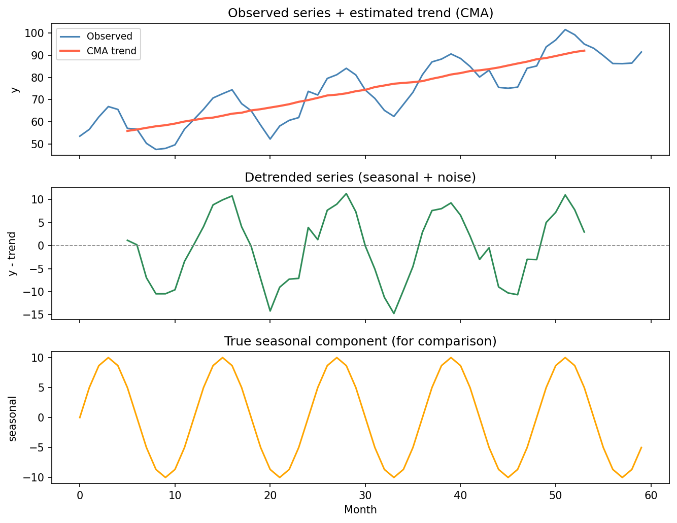
The red CMA line smooths away the wiggles; subtracting it leaves the seasonal wave (middle), which matches the true component (bottom).
What you see: the red CMA line follows the blue observed series at a distance, smoothing away the wiggles. The green detrended panel oscillates around zero — that regular wave is the seasonal pattern, and the slight irregularity in it is the noise. The orange panel shows the true seasonal component for comparison; the green matches it closely.
Using statsmodels for full decomposition
The manual CMA gives you the intuition. In practice, statsmodels wraps the same logic (and improvements like STL) in one function call. Here it is on the exact same synthetic series, given a monthly DatetimeIndex:
import pandas as pd
from statsmodels.tsa.seasonal import seasonal_decompose

# Same y as above, now a pandas Series indexed by month
idx = pd.date_range("2021-01-01", periods=60, freq="MS")
ys = pd.Series(y, index=idx)

result = seasonal_decompose(ys, model="additive", period=12)
result.plot()   # draws the four-panel figure below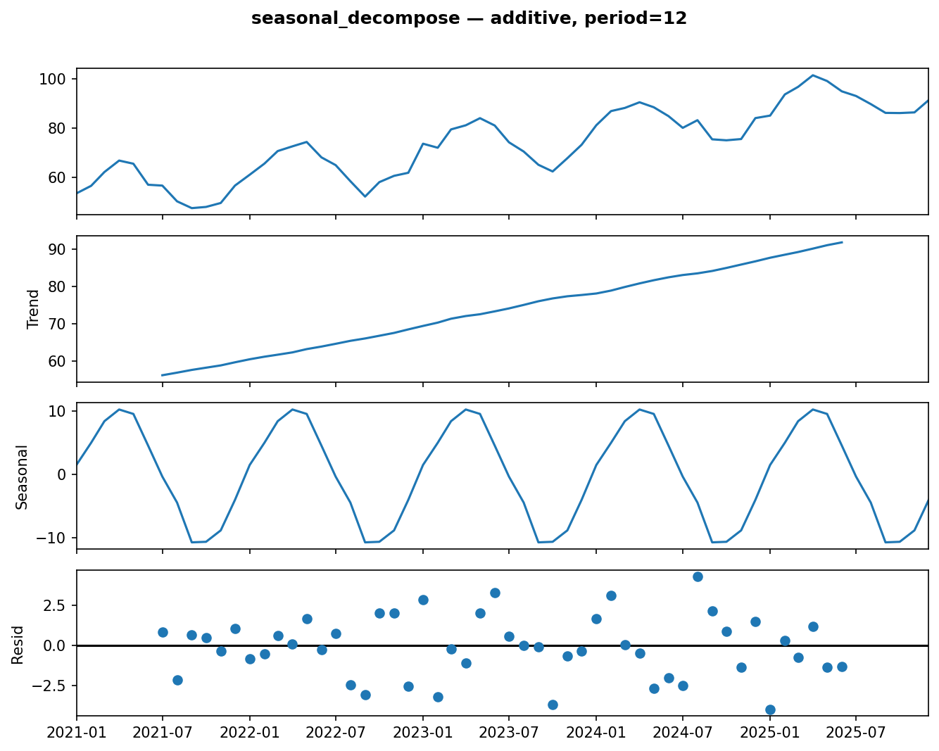
One call splits the series into Observed, Trend, Seasonal, and Residual. The clean upward Trend, the regular ±10 Seasonal wave, and the structureless Residual confirm an additive fit.
result.trend, result.seasonal, and result.resid are each a Series you can inspect individually. The residual panel scattering randomly around zero — with no leftover wave — is the sign of a good fit. Pass model="multiplicative" if your seasonal amplitude grows with the level.
In one breath
Every series is layered from a few simpler stories: a trend (long-run direction), seasonality (a
pattern repeating on a fixed calendar period), longer cycles (variable-length, usually folded into
trend at this stage), and the residual (what’s left — ideally white noise; leftover structure means
unmodelled signal). Decide additive (y = T + S + R, seasonal swing a fixed amount) vs
multiplicative (y = T × S × R, swing grows with the level) by eye — and if multiplicative, take a
log first to make it additive. A centered moving average with window = the seasonal period estimates
the trend (cancelling the seasonal peaks/troughs); subtract it to expose seasonal + noise.
statsmodels.seasonal_decompose does all of this in one call.
Practice
Quick check
A question to carry forward
Decomposition let you see the trend — that clean upward ramp in the second panel. But seeing it and modelling it are different problems. The workhorse forecasting model, ARIMA, refuses to fit a series whose mean keeps drifting upward; it needs the trend gone, not just identified. Decomposition diagnosed the patient; it didn’t treat them.
So the question to carry forward is: how do you formally test whether a series’ mean and variance are
stable over time — and, when they aren’t, how do you transform the series until they are? The next lesson,
stationarity, ADF and differencing, defines exactly what “stationary” means, gives you the Augmented
Dickey-Fuller test to check it with a single p-value, and shows how differencing (the d in ARIMA)
strips the trend out so the classical models can finally do their work.
Practice this in an interview
All questionsDecomposition separates a series into a trend component (long-run direction), a seasonal component (periodic, fixed-period pattern), and a residual (everything left over). Additive decomposition sums the three; multiplicative decomposition multiplies them, which is appropriate when seasonal swings grow with the level.
Shuffling destroys temporal order, so the model trains on future data and is evaluated on the past — a direct information leak. Time series observations are serially correlated, meaning past values predict future ones, and any random split obliterates that structure entirely.
Simple exponential smoothing computes a weighted average of all past observations where weights decay geometrically, controlled by a single smoothing parameter alpha. Holt's method adds a trend component with a second parameter beta; Holt-Winters (ETS) adds a seasonal component with a third parameter gamma, making it a strong baseline for series with both trend and seasonality.
Prophet is a curve-fitting model that decomposes the series into trend, seasonality, and holidays; it handles missing data, multiple seasonalities, and non-uniform time grids with minimal tuning and is accessible to non-statisticians. ARIMA is a statistical model based on autocorrelation structure; it is more appropriate when the series is short, noise is small, and you need principled uncertainty intervals from an explicit stochastic process.