Stationarity, ADF & differencing
ARIMA keeps demanding a 'stationary' series. What does that mean, how do I check it, and how do I make my data stationary?
What you'll learn
- Stationarity: why ARIMA needs constant mean, variance, and autocovariance over time
- How to check stationarity — rolling statistics and the Augmented Dickey-Fuller test
- Differencing and log transforms to make a non-stationary series stationary
Before you start
Decomposition let you see the trend, but ARIMA can’t fit a series whose mean keeps drifting — it needs the trend gone. This lesson is the treatment that follows that diagnosis: what “stationary” precisely means, the one test that checks it, and the transform that gets you there.
What stationarity means
A time series is stationary when its statistical properties don’t change as time moves forward. Formally, three things must hold across all time windows of the same length:
- Mean — the average level stays roughly constant.
- Variance — the spread of values stays roughly constant.
- Autocovariance — the relationship between a value and its own past (its correlation structure) depends only on the lag, not on the absolute position in time.
A sales series that grows every year violates the first condition — its mean is drifting upward. A price series during a volatile crisis violates the second — variance explodes, then calms. ARIMA and most classical forecasting models assume the series it is learning from is stationary, because they try to model a stable, repeatable dynamic. If the mean keeps shifting, there is no stable dynamic to learn: the model’s coefficient estimates change depending on which time window you fit on, and forecasts diverge quickly.
A visual
The SVG below shows the contrast directly. The left panel has a drifting mean — classic non-stationarity. The right panel has a flat mean, constant spread, and no trend.
Left: a trending (non-stationary) series — mean drifts upward over time. Right: a stationary series — mean and spread are stable across the window.
How to check: rolling statistics and the ADF test
There are two complementary approaches. Start visual, then confirm statistically.
Visual check — rolling mean and standard deviation
Compute a rolling window mean and standard deviation and plot them alongside the original series. If the rolling mean is flat and the rolling std is roughly constant, the series looks stationary. If either drifts systematically, you have a problem. This is a quick sanity check, not a formal test.
The Augmented Dickey-Fuller test
The Augmented Dickey-Fuller (ADF) test is the standard statistical test for a unit root — the formal term for the kind of non-stationarity caused by a trend. The terminology needs unpacking:
- Unit root — a particular structure in the time series model that causes the series to wander indefinitely rather than mean-revert. A random walk (
y_t = y_{t-1} + noise) has a unit root. - Null hypothesis of ADF — the series has a unit root (i.e., it is non-stationary). This is the opposite of what you want.
- Alternative hypothesis — the series does not have a unit root (i.e., it is stationary).
So a small p-value (say, below 0.05) means you reject the null — the series is stationary. A large p-value means you fail to reject — the series likely has a unit root and needs treatment.
The test lives in statsmodels:
from statsmodels.tsa.stattools import adfuller

result = adfuller(series)
print(f"ADF statistic : {result[0]:.4f}")
print(f"p-value       : {result[1]:.4f}")
print(f"Critical vals : {result[4]}")
Run it on the trending series we build below (a linear drift plus noise) and then on its first difference, and the verdict flips cleanly:
ADF original : stat= 2.0239   p=0.9987     # huge p → fail to reject → non-stationary
ADF diff(1)  : stat=-5.8246   p=0.0000     # tiny p, stat well below the 5% crit (-2.89) → stationary
The output includes the ADF statistic (more negative = stronger evidence of stationarity), the p-value, and critical values at 1%, 5%, and 10% significance levels. The original series scores p = 0.9987 — about as non-stationary as it gets. One difference drops it to p ≈ 0, with the statistic far below the 5% critical value. That is exactly the transition you are aiming for.
Making a series stationary: differencing
If the series has a trend (non-constant mean), the standard fix is differencing. The first difference of a series replaces each value with the change since the previous step:
diff1 = series.diff().dropna()This removes a linear trend. If the trend is quadratic or the first difference still drifts, apply a second difference — but see the warning below.
For seasonality, seasonal differencing subtracts the value from the same period in the prior cycle. For monthly data with yearly seasonality:
diff_seasonal = series.diff(12).dropna()Stabilizing variance with a log transform
If the series shows growing variance — the swings get larger as the level rises, common in revenue or stock prices — a log transform compresses that before you difference:
import numpy as np
log_series = np.log(series)
log_diff = log_series.diff().dropna()
The log transform converts multiplicative growth patterns into additive ones, which differencing can then remove.
The d in ARIMA
ARIMA(p, d, q) has three components. The middle one, d, is the order of differencing — how many times you apply .diff() before passing the series to ARIMA. d=0 means the series is already stationary. d=1 is the most common value and handles most linear trends. d=2 is occasionally needed and rarely anything higher.
Playground: watch the trend vanish
The code below builds a trending series (constant drift plus noise), plots the original and the first difference side by side, and prints their rolling means so you can compare. The trend should disappear after differencing.
import numpy as np
import pandas as pd
import matplotlib.pyplot as plt

np.random.seed(0)
n = 120
t = np.arange(n)

# Trending series: linear drift + random noise
drift = 0.5
noise = np.random.normal(0, 1, n)
series = pd.Series(10 + drift * t + noise, name="original")

# First difference
diff1 = series.diff().dropna()
diff1.name = "first difference"

# Rolling mean (window = 20)
roll_orig = series.rolling(20).mean()
roll_diff = diff1.rolling(20).mean()

fig, axes = plt.subplots(2, 1, figsize=(8, 6), sharex=False)

axes[0].plot(series.values, color="#6366f1", lw=1.5, label="series")
axes[0].plot(roll_orig.values, color="#ef4444", lw=2, linestyle="--", label="rolling mean")
axes[0].set_title("Original (trending)")
axes[0].legend(fontsize=9)
axes[0].set_ylabel("value")

axes[1].plot(diff1.values, color="#6366f1", lw=1.5, label="diff(1)")
axes[1].plot(roll_diff.values, color="#22c55e", lw=2, linestyle="--", label="rolling mean")
axes[1].axhline(0, color="#9ca3af", lw=1)
axes[1].set_title("After first difference (trend removed)")
axes[1].legend(fontsize=9)
axes[1].set_ylabel("change")
axes[1].set_xlabel("time step")

plt.tight_layout()
plt.show()

print(f"Original   — mean: {series.mean():.2f}, std: {series.std():.2f}")
print(f"Diff(1)    — mean: {diff1.mean():.2f}, std: {diff1.std():.2f}")
Original — mean: 39.88, std: 17.47
Diff(1) — mean: 0.49, std: 1.46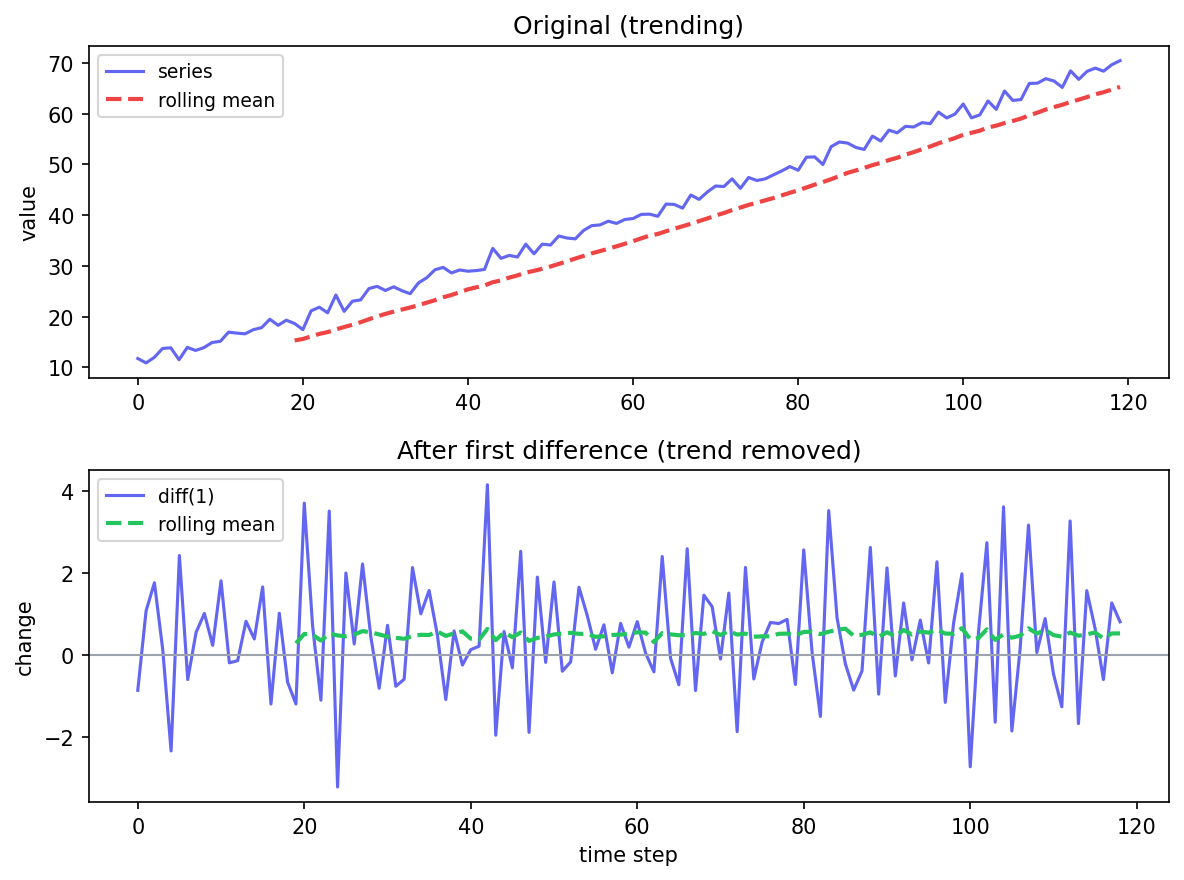
Top: the original’s rolling mean marches upward (mean 39.88). Bottom: after one difference the mean is flat at 0.49 — almost exactly the 0.5 drift, the hallmark of a stationary series.
There’s the prediction answer: the differenced mean is 0.49, essentially the 0.5 drift per step, and the bottom panel hovers around zero with a roughly constant spread — no long upward march. That is what the ADF p-value (0.0000 after differencing) confirms statistically.
Putting it all together: a workflow
- Plot the raw series and its rolling mean/std. Does the mean drift? Does variance grow?
- If yes, apply a log transform first if variance is growing, then difference.
- Run
adfulleron the result. If the p-value is above 0.05, difference once more. - Stop as soon as the p-value is small. Note how many times you differenced — that is
din ARIMA. - Before modelling, look at the ACF and PACF of the stationary series to choose
pandq.
In one breath
A series is stationary when its mean, variance, and autocovariance stay constant over time — and
classical models like ARIMA demand it, because a drifting mean has no stable dynamic to learn. Check it
two ways: eyeball a rolling mean/std (flat = good), then confirm with the Augmented Dickey-Fuller
test, whose null is “has a unit root (non-stationary)” — so a small p-value (< 0.05) means stationary
(our trending series: p = 0.9987 → after one difference p ≈ 0). The cure for a drifting mean is
differencing (series.diff()), which is exactly the d in ARIMA(p, d, q); for growing variance,
take a log first, then difference; for seasonality, use a seasonal difference diff(period). Difference
the minimum number of times — over-differencing injects a tell-tale negative ACF spike at lag 1.
Practice
Quick check
A question to carry forward
You’ve now got a stationary series and a number — d, how many times you differenced. But ARIMA has two
more knobs: p and q. The over-differencing warning even hinted at how to read them (“a large negative
spike at lag 1 in the ACF”). Those two letters — ACF and PACF — keep appearing, and they’re how you
actually choose the model orders instead of guessing.
So the question to carry forward is: once a series is stationary, how do you look at its internal
correlation structure to decide how many autoregressive (p) and moving-average (q) terms it needs?
The next lesson, ACF and PACF, reads the autocorrelation and partial-autocorrelation plots like a
fingerprint — a sharp cutoff here, a slow decay there — to point you straight at the right ARIMA orders.
Practice this in an interview
All questionsA stationary series has a constant mean, constant variance, and autocovariance that depends only on lag — not on when you look. Most classical models (ARIMA, VAR) require it. The Augmented Dickey-Fuller (ADF) test is the standard check; a p-value below 0.05 lets you reject the unit-root null and conclude the series is stationary.
Choose d by differencing until the ADF test confirms stationarity; choose p from the PACF cutoff and q from the ACF cutoff on the differenced series; then confirm with AIC or BIC to guard against over-fitting. In practice, an automated grid search over a small range of candidates with information criteria is more reliable than visual inspection alone.
ARIMA(p,d,q) models non-seasonal series by combining autoregression, differencing, and a moving average of errors. SARIMA extends it with a second set of seasonal parameters (P,D,Q,s) that operate at the seasonal lag s, handling periodic patterns that ARIMA alone cannot capture.
A Vector Autoregression (VAR) model extends ARIMA to multiple time series simultaneously: each variable is regressed on its own past values and the past values of all other variables in the system. Use VAR when the series have mutual predictive relationships (Granger-causality) and you want to model those interactions; ARIMA is sufficient when one series can be forecast in isolation.