Exponential smoothing & Holt-Winters
Learn how Simple Exponential Smoothing, Holt's method, and Holt-Winters build up a fast, robust forecaster by weighting recent data more heavily — and when this ETS family beats ARIMA.
What you'll learn
- How SES weights recent observations exponentially so that older data fades smoothly into the past
- How Holt's method adds a trend component (beta) and Holt-Winters adds seasonality (gamma)
- ETS vs ARIMA: when to reach for each, and why strong clear seasonality often tips the balance
Before you start
The classical chapter ended on a complaint: ARIMA and VAR are powerful but heavy — stationarity tests, order hunts, residual diagnostics, all per series. This chapter opens the lighter path, and this lesson is the first model on it.
No — you don’t always need full ARIMA. The exponential smoothing family, also called ETS (Error-Trend-Seasonal), is a collection of models that are fast to fit, easy to interpret, and surprisingly competitive with ARIMA on real-world data. The core idea is beautifully simple: weight observations so that the most recent value matters most and every older value matters a little less, with the influence decaying exponentially into the past.
Simple Exponential Smoothing (SES)
Simple Exponential Smoothing produces a forecast by maintaining a single running estimate called the level, updated after every new observation.
The recursive update rule is:
level_t = alpha * y_t + (1 - alpha) * level_(t-1)
y_tis the observed value at timet.level_(t-1)is the level estimate from the previous step — a smoothed summary of all earlier history.- alpha (the smoothing parameter) lives in the interval
(0, 1)and controls how fast the memory fades.
When alpha is close to 1, the level lunges toward each new observation — the model is reactive but noisy. When alpha is close to 0, the level barely moves — the model is stable but slow to track genuine shifts. The one-step-ahead forecast is simply the current level: forecast_(t+1) = level_t.
Why this is genuinely exponential
Unrolling the recursion shows what is happening under the hood. The current level is:
level_t = alpha * y_t + alpha*(1-alpha)*y_(t-1) + alpha*(1-alpha)^2*y_(t-2) + ...
Every additional lag picks up another factor of (1-alpha). Because (1-alpha) is less than 1, those factors shrink toward zero — an exponential decay of weights as you look further into the past. The diagram below shows this visually.
alpha * (1-alpha)^k for lag k. With alpha = 0.4, the most-recent observation carries 40 % of the weight; three lags back it is down to about 14 %.Holt’s method — adding a trend
Holt’s method (also called double exponential smoothing) extends SES by tracking two quantities:
- Level
l_t— the smoothed baseline, updated with smoothing parameter alpha. - Trend
b_t— the smoothed slope (rate of change), updated with smoothing parameter beta.
The forecast h steps ahead is l_t + h * b_t: start from the current level and project along the current trend. Beta, like alpha, lives in (0, 1) and controls how quickly the model revises its trend estimate.
Holt-Winters — adding seasonality
Holt-Winters (also called triple exponential smoothing) adds a third set of smoothed quantities: seasonal indices s_t, one for each period within the season (twelve values for monthly data with annual seasonality, seven for daily data with weekly seasonality).
A third smoothing parameter gamma controls how fast the seasonal indices adapt. The seasonal_periods parameter tells the model the length of one seasonal cycle.
There are two variants:
- Additive — the seasonal component is added to the level. Use this when the size of seasonal swings stays roughly constant regardless of the level of the series.
- Multiplicative — the seasonal component multiplies the level. Use this when seasonal swings grow proportionally as the level rises (common in retail and tourism data).
Together the three parameters — alpha for level, beta for trend, gamma for seasonality — define what the forecasting community calls the ETS (Error-Trend-Seasonal) model family. The “E” refers to the error structure (additive or multiplicative), and every combination of (E, T, S) specification is a distinct model in the family.
Implement SES by hand
import numpy as np
import matplotlib.pyplot as plt

np.random.seed(0)

# Simulate a noisy series with a gradual upward drift
n = 60
time = np.arange(n)
series = 10 + 0.3 * time + np.random.randn(n) * 2.5

def ses(y, alpha):
    """Return the level (smoothed) series for a given alpha."""
    level = np.empty(len(y))
    level[0] = y[0]          # initialise with the first observation
    for t in range(1, len(y)):
        level[t] = alpha * y[t] + (1 - alpha) * level[t - 1]
    return level

level_high = ses(series, alpha=0.8)   # reactive
level_low  = ses(series, alpha=0.1)   # stable

fig, ax = plt.subplots(figsize=(9, 4))
ax.plot(time, series,     color="gray",  alpha=0.5, label="observed")
ax.plot(time, level_high, color="#e07b39", linewidth=2, label="SES alpha=0.8 (reactive)")
ax.plot(time, level_low,  color="#4c9be8", linewidth=2, label="SES alpha=0.1 (stable)")
ax.set_xlabel("Time"); ax.set_ylabel("Value")
ax.set_title("Simple Exponential Smoothing — effect of alpha")
ax.legend()
plt.tight_layout()
plt.show()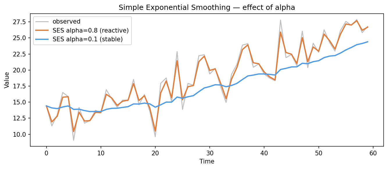
High alpha (orange, 0.8) hugs every bump; low alpha (blue, 0.1) glides smoothly past the noise — and lags genuine shifts.
The orange line (alpha=0.8) hugs every bump in the data, while the blue line (alpha=0.1) glides smoothly past most of the noise. Neither is universally better — the right alpha depends on how much of the observed variability is signal versus noise. (For a volatile stock you’d usually want the smoother low-alpha line; for a baseline that genuinely shifts, the reactive high-alpha one.)
Fitting Holt-Winters with statsmodels
For production use you should let statsmodels fit the smoothing parameters automatically by minimizing the sum of squared one-step forecast errors.
from statsmodels.tsa.holtwinters import ExponentialSmoothing
import pandas as pd

# Assume `series` is a pandas Series with a DatetimeIndex and freq="MS"
model = ExponentialSmoothing(
    series,
    trend="add",            # additive trend (use "mul" for multiplicative)
    seasonal="add",         # additive seasonality
    seasonal_periods=12,    # 12 months per year
)
fit = model.fit()

forecast = fit.forecast(steps=12)   # 12-month horizon
print(fit.summary())On a monthly series with a clear yearly cycle, the additive Holt-Winters forecast carries the trend and the season forward — no differencing, no order hunt, one model call:
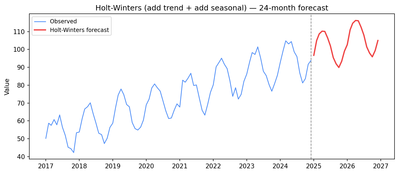
Holt-Winters (additive trend + additive seasonal): the 24-month forecast extends both the trend and the yearly cycle — like SARIMA, but with no stationarity tests or ACF/PACF hunt.
That is the appeal of the ETS family in one picture: a forecast that respects trend and seasonality, produced from three interpretable smoothing knobs that statsmodels tunes for you.
When ETS beats ARIMA
Both ARIMA and ETS are serious, widely-used forecasters. The practical rule of thumb:
| Situation | Lean toward |
|---|---|
| Strong, clear seasonality | ETS (Holt-Winters) |
| Many series to forecast automatically | ETS (fewer assumptions to tune) |
| Complex autocorrelation structure in residuals | ARIMA |
| Irregular, non-calendar-aligned data | ARIMA |
| Speed and interpretability matter most | ETS |
ETS tends to shine when the seasonal pattern is stable and predictable — monthly retail, yearly energy demand, weekly call-center volume. ARIMA tends to win when the dynamics are driven by lagged shocks rather than a smooth underlying level-plus-trend-plus-season structure. In practice, the best strategy is to fit both and compare out-of-sample error on a held-out validation window.
In one breath
The exponential smoothing / ETS family forecasts by weighting recent observations more than old ones,
decaying exponentially into the past. Simple Exponential Smoothing tracks one level updated as
level_t = alpha·y_t + (1−alpha)·level_(t−1) — high alpha is reactive-but-jumpy, low alpha is smooth-but-laggy
— and forecasts a flat line, so it has no trend or seasonality. Holt’s method adds a smoothed trend
(parameter beta); Holt-Winters adds seasonal indices (parameter gamma, plus seasonal_periods),
in additive or multiplicative form. Together (alpha, beta, gamma) define the ETS family, and statsmodels
optimises them for you. Reach for ETS over ARIMA when seasonality is strong and clear or when you must
forecast many series fast; reach for ARIMA when the dynamics live in lagged shocks — and when unsure, fit
both and compare on a held-out window.
Practice
Quick check
A question to carry forward
ETS made forecasting lighter — three knobs, fitted automatically. But it still assumes a tidy world: one clean seasonal period, a smooth level-plus-trend, no awkward gaps or one-off events. Real business series are messier. They often have two seasonalities at once (weekly and yearly), irregular holidays that don’t sit on a fixed lag, missing days, and abrupt level shifts when a product relaunches.
So the question to carry forward is: is there a forecaster built for that mess — one a non-specialist can point at a raw daily series and get a sensible, holiday-aware forecast without tuning anything? The next lesson is Prophet, Meta’s decomposition-based model designed for exactly these business time series: multiple seasonalities, a built-in holiday calendar, robustness to gaps and outliers, and interpretable trend-changepoints — forecasting for people who don’t want to become time-series experts first.
Practice this in an interview
All questionsSimple exponential smoothing computes a weighted average of all past observations where weights decay geometrically, controlled by a single smoothing parameter alpha. Holt's method adds a trend component with a second parameter beta; Holt-Winters (ETS) adds a seasonal component with a third parameter gamma, making it a strong baseline for series with both trend and seasonality.
Prophet is a curve-fitting model that decomposes the series into trend, seasonality, and holidays; it handles missing data, multiple seasonalities, and non-uniform time grids with minimal tuning and is accessible to non-statisticians. ARIMA is a statistical model based on autocorrelation structure; it is more appropriate when the series is short, noise is small, and you need principled uncertainty intervals from an explicit stochastic process.
Decomposition separates a series into a trend component (long-run direction), a seasonal component (periodic, fixed-period pattern), and a residual (everything left over). Additive decomposition sums the three; multiplicative decomposition multiplies them, which is appropriate when seasonal swings grow with the level.
ARIMA(p,d,q) models non-seasonal series by combining autoregression, differencing, and a moving average of errors. SARIMA extends it with a second set of seasonal parameters (P,D,Q,s) that operate at the seasonal lag s, handling periodic patterns that ARIMA alone cannot capture.