Naive Bayes
Bayes' rule plus one bold assumption — that features are independent — gives a fast, surprisingly strong classifier, especially for text. Learn the arithmetic, smoothing, log-space scoring, useful variants, and the failure modes that matter in production.
What you'll learn
- How Bayes' rule turns class priors and feature evidence into a prediction
- Why conditional independence makes a huge joint probability practical to estimate
- How Laplace smoothing prevents one unseen feature from destroying a class score
- Why Naive Bayes probabilities are often overconfident, and when another model is better
Before you start
At 3:02 a.m., your support system receives an email:
“Free prize now. Click this link to claim your money.”
A spam filter has milliseconds to decide. It has a few thousand labeled emails, a vocabulary of perhaps 100,000 words, and no realistic chance of seeing every possible combination of words during training.
It still needs an answer.
Naive Bayes gets one by combining Bayes’ rule with a deliberately crude shortcut: treat the features as independent once you know the class. That shortcut is usually false. It is also remarkably useful.
Bayes’ rule, applied to classification
A class is the label we want to predict, such as spam or ham. A feature is an observed piece of evidence, such as the word prize.
Bayes’ rule says:
P(class | features) ∝ P(class) × P(features | class)
                   posterior   prior     likelihood
The posterior is the probability of a class after seeing the email. The prior is how common that class was beforehand. The likelihood is how probable the observed features are under that class.
Calculate the right-hand side for each class and choose the largest score. The ∝ means the score is not normalized. For two classes:
P(spam | features)
  = spam score / (spam score + ham score)
The denominator is the same for every class, so you can skip it when choosing a winner. If you need a probability to show a user or make a risk decision, normalize.
The difficult term is P(features | class). For a long email, this is the probability of the entire observed word combination. A training set may contain free, prize, and now separately but never that exact combination. This is the joint probability problem: the number of possible combinations grows rapidly, making each combination sparse.
The “naive” leap
Naive Bayes assumes the features are conditionally independent: after fixing the class, knowing one feature gives you no additional information about another.
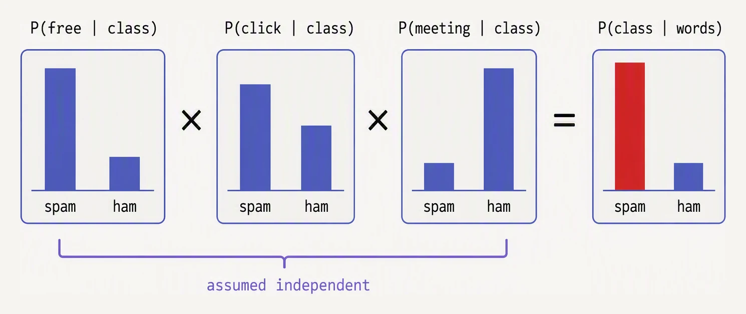
“Naive” is the assumption that the features do not talk to each other.
That does not mean the features are independent in general. free and prize may appear together because both are common in spam. Naive Bayes simply pretends that, once considering spam, seeing free does not change the probability of prize.
The joint likelihood becomes a product:
P(features | C)
  = P(f₁ | C) × P(f₂ | C) × P(f₃ | C) × …
C is the class, and f₁, f₂, and so on are the features. Each term can now be estimated from counts. For a word-count model:
P(word | C)
  = count of that word in class C / total word count in class C
If a word occurs twice, its evidence appears twice. With word counts xⱼ, the Multinomial Naive Bayes score is:
P(C) × ∏ⱼ P(wordⱼ | C)ˣʲThe product repeats a word’s contribution according to its count.
A worked classification
Use the suspicious email fragment “free prize now”. Suppose training produced these class-conditional word probabilities:
| word | likelihood if spam | likelihood if ham |
|---|---|---|
| free | 0.40 | 0.02 |
| prize | 0.30 | 0.01 |
| now | 0.20 | 0.10 |
Assume the classes are equally common:
P(spam) = 0.5
P(ham)  = 0.5
The unnormalized scores are:
spam: 0.5 × 0.40 × 0.30 × 0.20 = 0.012
ham:  0.5 × 0.02 × 0.01 × 0.10 = 0.00001
Normalize them:
P(spam | email)
  = 0.012 / (0.012 + 0.00001)
  ≈ 0.999
The classifier calls it spam. It never estimated the probability of the complete phrase; it multiplied three easier estimates.
The prior matters too. If spam makes up only 1 percent of incoming mail, the likelihood evidence favors spam by:
(0.40 / 0.02) × (0.30 / 0.01) × (0.20 / 0.10)
  = 20 × 30 × 2
  = 1200
The prior odds are 0.01 / 0.99, or about 0.0101. Multiplying by 1200 gives posterior odds of about 12.1, or a spam probability near 0.924. The message is still probably spam, but less confidently. A rare class needs stronger evidence.
Smoothing: stopping one zero from winning
Imagine prize never appeared in the ham messages:
P(prize | ham) = 0The entire ham product becomes zero. One unseen word is treated as absolute proof, even though the training set was merely finite.
Laplace smoothing, also called add-one smoothing, adds a small count to every word:
P(word | C)
  = (N(word, C) + α) / (N(C) + αV)
Here:
N(word, C)is the observed count of the word in classC.N(C)is the total count of all words in classC.Vis the vocabulary size.αis the smoothing amount.
With α = 1, a zero count gets a nonzero probability. The denominator also increases because every vocabulary word received the extra count. Both parts must be adjusted, or the probabilities will not form a valid distribution.
Larger α values flatten probabilities more aggressively. That can help with tiny datasets but can also wash out useful frequency differences. Smoothing guards against brittle zeros; it does not make the model smarter.
Why the arithmetic moves to log-space
A document can produce an extremely small product. If an email contains 200 words and each likelihood is around 0.001, the product is around 10⁻⁶⁰⁰, which can underflow to zero in ordinary floating-point arithmetic.
Logs turn multiplication into addition:
log score(C)
  = log P(C) + Σⱼ xⱼ log P(wordⱼ | C)
The winning class does not change because the logarithm is monotonic. Compare sums instead of multiplying tiny numbers. To normalize log scores, use a numerically stable log-sum-exp calculation rather than exponentiating very negative values first.
MultinomialNB handles smoothing and log-domain scoring internally.
A small working classifier
This pipeline learns its vocabulary during fit, converts messages into word counts, and fits Multinomial Naive Bayes:
from sklearn.feature_extraction.text import CountVectorizer
from sklearn.naive_bayes import MultinomialNB
from sklearn.pipeline import make_pipeline

texts = [
    "win free money now",
    "free entry winner",
    "team meeting at noon",
    "project update attached",
    "claim your prize free",
    "lunch tomorrow",
    "urgent click this link",
    "review the report please",
]
labels = [1, 1, 0, 0, 1, 0, 1, 0]  # 1 = spam, 0 = ham

model = make_pipeline(
    CountVectorizer(),
    MultinomialNB(),
)
model.fit(texts, labels)

for text in ["free prize click now", "meeting about the project"]:
    prediction = model.predict([text])[0]
    label = "SPAM" if prediction == 1 else "HAM"
    print(label, "->", repr(text))
SPAM -> 'free prize click now'
HAM -> 'meeting about the project'The word about was not in the fitted vocabulary, so the vectorizer ignores it. The other words provide enough evidence for HAM in this tiny example.
Keeping the vectorizer and classifier in one pipeline also prevents preprocessing leakage. Fit transformations only on training data, then evaluate with a proper split or cross-validation. See train, test, and cross-validation and the scikit-learn API.
Why a wrong assumption can still classify well
Compare two classes in log-space:
log score(spam) - log score(ham)
  = log prior ratio
    + Σⱼ xⱼ log likelihood ratioⱼ
Every word contributes evidence. A word common in spam adds a positive amount; one common in ham adds a negative amount. Classification only needs the total to have the correct sign.
Correlated words can inflate the total without changing its sign. If free and prize tend to arrive together, Naive Bayes counts their evidence as two independent discoveries. The ranking can remain correct even while the probability becomes overconfident.
This explains the Naive Bayes surprise:
- its probability estimates can be poor;
- its class ranking can still be useful;
- it is cheap to train and score at scale.
The assumption fails more seriously when the class depends on interactions. “Not expensive” and “not refundable” can mean something different from either phrase alone. N-grams capture some local phrases but increase vocabulary sparsity. Naive Bayes does not understand syntax, negation, sarcasm, or meaning like a language model.
Which Naive Bayes variant fits the features?
The distributional assumption should match the representation.
| Situation | Reasonable first choice | What it assumes |
|---|---|---|
| Word or token counts | MultinomialNB | Repeated occurrences contribute repeated evidence |
| Binary word presence | BernoulliNB | Presence and absence carry evidence |
| Continuous measurements | GaussianNB | Each feature is approximately normal within a class |
| Strongly imbalanced text classes | ComplementNB as an experiment | Complement statistics may reduce some imbalance problems |
For text, MultinomialNB is usually the natural first choice for counts or nonnegative weights. BernoulliNB can behave differently on short messages because it models both word presence and absence. GaussianNB is not a default for sparse bag-of-words data: word counts are not bell-shaped continuous measurements.
A practical baseline often compares Naive Bayes with logistic regression. Logistic regression may provide a better boundary and probability behavior after tuning; Naive Bayes trains quickly and exposes count-based evidence. For semantic similarity or long-range context, a transformer is more capable but costs more money, memory, latency, and operational attention. The cheap baseline shows whether that expense is necessary.
Failure modes you can see in production
“The model predicts ham for almost everything”
A confusion matrix may show excellent accuracy and almost no detected spam. If 99 percent of training messages are ham, the learned prior strongly favors ham, and an always-ham classifier gets 99 percent accuracy.
Use precision, recall, and a cost-aware threshold rather than accuracy alone; picking the right metric explains why. You can supply class priors or change the threshold, but do not automatically force equal priors. If production really is 99 percent ham, discarding that information may create too many false alarms.
“The model says 0.99, but many 0.99 predictions are wrong”
Correlated features can look like independent votes, making probabilities too extreme even when rankings remain useful.
Measure calibration: among predictions near 0.9, roughly 90 percent should be correct if probabilities are well calibrated. If they are not, calibrate on data separate from the data used to fit the classifier, and validate carefully on small datasets. Read model calibration before using a Naive Bayes probability as a financial risk, safety score, or automatic escalation rule.
A threshold of 0.5 is not sacred. Lower it when false negatives are expensive; raise it when false positives have a higher cost.
“A new campaign sails through the filter”
A sudden recall drop often indicates vocabulary drift. A new campaign may use images, deliberate misspellings, or unfamiliar product names.
Inspect the vectorizer’s unknown-token rate and compare current word frequencies with training frequencies. Retrain with recent labeled examples, and keep a time-based evaluation set so a random split does not hide the change. Naive Bayes is easy to retrain, but a poisoned batch of mislabeled messages can shift its counts quickly.
When to use it, and when not to
Use Naive Bayes when input is high-dimensional and sparse, labels are available, training must be cheap, and a strong baseline matters. Spam filtering, ticket routing, language identification, and rough topic tagging are classic fits.
Do not use it merely because the output is called a probability. Its probabilities are often the weak part. Avoid relying on it alone when feature interactions carry the meaning, calibrated risk is central, or the representation discards useful context.
Build it early, measure it with the metric that reflects the cost of mistakes, inspect its errors, and keep it if speed and simplicity win. Replace it when the errors reveal a limitation that more arithmetic cannot fix.
In one breath
- Bayes’ rule combines a prior with a likelihood to score each class.
- Naive Bayes assumes features are conditionally independent given the class, turning one difficult joint probability into a product.
- The product can rank classes well even when its probabilities are wrong.
- Laplace smoothing prevents an unseen class-specific word from creating a zero score. Log-space turns unstable products into stable sums.
MultinomialNBfits word counts,BernoulliNBfits binary presence, andGaussianNBfits continuous features with a normality assumption.- It is a fast baseline, not a semantic model; check its confidence rather than admiring it.
Quick check
Quick check
Next
A single model is only the beginning. The next step is combining models: bagging, boosting & stacking.
Practice this in an interview
All questionsNaive Bayes multiplies feature likelihoods, so one unseen feature-class combination with probability zero makes the entire class score zero. Laplace or Lidstone smoothing adds a positive pseudocount to every possible value; log probabilities prevent underflow but do not replace smoothing.
Naive Bayes is called naive because it assumes features are conditionally independent given the class, an assumption that is rarely literally true for words. It remains effective for text because the factorized model is fast and data-efficient for high-dimensional sparse inputs, and its approximate scores often still rank the correct class highest even when its probabilities are overconfident.
Naive Bayes applies Bayes' theorem to classify by computing the posterior probability of each class given the features. It is naive because it assumes all features are conditionally independent given the class label — an assumption that is almost never true in practice, yet the classifier still works surprisingly well for text and other sparse data.
Bagging trains many independent models in parallel on bootstrap samples and averages them, which mainly reduces variance; boosting trains models sequentially so each corrects its predecessor's errors, which mainly reduces bias. Use bagging when the base learner is high-variance and overfits; use boosting when you need to reduce underfitting and maximise accuracy, accepting more tuning and overfitting risk.