Class imbalance
When 99% of your rows are one class, "always predict negative" hits 99% accuracy and ships nothing useful. Here's how to actually fix it.
Written and reviewed by Shreyash Prashu Last reviewed
What you'll learn
- How to detect imbalance and why accuracy lies about it
-
class_weight='balanced'— the one-line fix that often wins - Resampling (RandomOverSampler, RandomUnderSampler, SMOTE) and what they really do
- Threshold tuning — usually the simplest and most underrated fix
Before you start
Most real classification problems are imbalanced. Fraud is rare. Churn is rare. Ad clicks are rare. Disease is rare. A naive classifier on a 99/1 dataset can hit 99% accuracy by predicting “negative” for every row — and catch zero of the positives that actually matter.
This lesson is about spotting that trap and getting out of it.
95% accuracy, 0 useful predictions — pick a strategy and watch recall move
The dataset below is 95% class 0 / 5% class 1. A model trained naively learns to always predict the majority class — high accuracy, worthless recall. Try each fix and see the confusion matrix change.
Train on the raw 95/5 split. The model learns to always predict the majority class — almost zero recall.
Detect the imbalance first
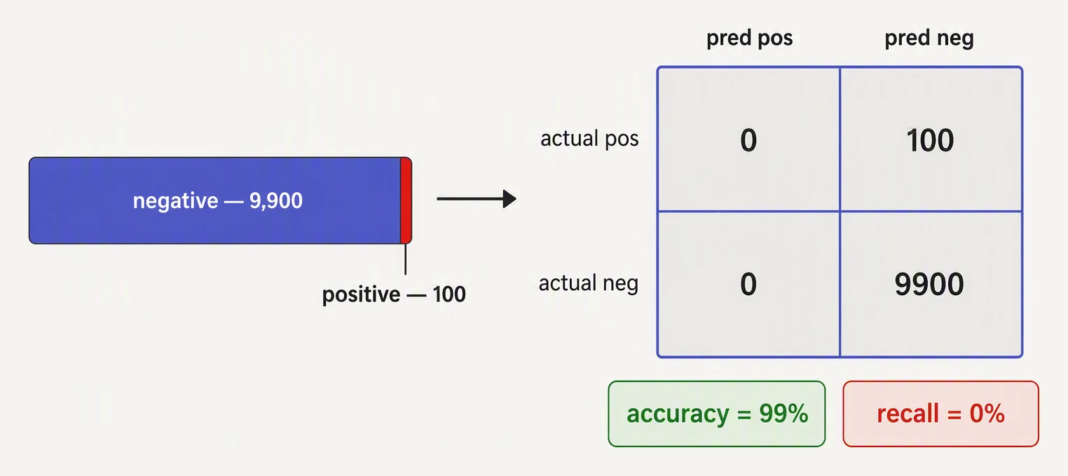
99% accurate and completely useless are compatible.
Before you reach for fancy techniques, look at the label distribution. One line of pandas tells you everything.
import numpy as np
import pandas as pd

from sklearn.datasets import make_classification

# Generate a 95/5 imbalanced churn-like dataset
X, y = make_classification(
    n_samples=4000, n_features=8, n_informative=5,
    weights=[0.95, 0.05],  # 95% non-churners, 5% churners
    random_state=0,
)
df = pd.DataFrame(X, columns=[f"f{i}" for i in range(8)])
df["churned"] = y

print("class counts:")
print(df["churned"].value_counts())
print("\nclass proportions:")
print(df["churned"].value_counts(normalize=True).round(3))
If the minority class is under 10% you’ve got imbalance worth handling. Under 1% and the problem is severe — most defaults will give you a model that ignores the minority entirely.
Why accuracy lies
import numpy as np

from sklearn.datasets import make_classification
from sklearn.linear_model import LogisticRegression
from sklearn.model_selection import train_test_split
from sklearn.metrics import accuracy_score, recall_score, precision_score, f1_score

X, y = make_classification(
    n_samples=4000, n_features=8, n_informative=5,
    weights=[0.95, 0.05], random_state=0,
)
X_tr, X_te, y_tr, y_te = train_test_split(X, y, test_size=0.3, stratify=y, random_state=0)

# Baseline: plain logistic regression, no rebalancing
clf = LogisticRegression(max_iter=1000).fit(X_tr, y_tr)
pred = clf.predict(X_te)

print(f"accuracy : {accuracy_score(y_te, pred):.3f}")
print(f"precision: {precision_score(y_te, pred, zero_division=0):.3f}")
print(f"recall   : {recall_score(y_te, pred):.3f}")
print(f"f1       : {f1_score(y_te, pred):.3f}")

# How often the model predicts each class:
print("predicted class counts:", np.bincount(pred))
Accuracy looks great. Recall is awful. Of all the actual churners, the model catches almost none — which is the entire reason you trained the model in the first place. Always report precision, recall, F1, and a confusion matrix on imbalanced problems. Accuracy is meaningless here.
Fix 1: class_weight='balanced' (the lazy win)
Most sklearn classifiers accept a class_weight argument. Setting it to
'balanced' automatically weights each class inversely proportional to
its frequency: a class that makes up 5% of rows gets 20× the loss
penalty of a class at 100%. No resampling, no extra dependencies, one
keyword argument.
from sklearn.datasets import make_classification
from sklearn.linear_model import LogisticRegression
from sklearn.model_selection import train_test_split
from sklearn.metrics import recall_score, precision_score, f1_score

X, y = make_classification(
    n_samples=4000, n_features=8, n_informative=5,
    weights=[0.95, 0.05], random_state=0,
)
X_tr, X_te, y_tr, y_te = train_test_split(X, y, test_size=0.3, stratify=y, random_state=0)

clf = LogisticRegression(max_iter=1000, class_weight="balanced").fit(X_tr, y_tr)
pred = clf.predict(X_te)
print(f"precision: {precision_score(y_te, pred):.3f}")
print(f"recall   : {recall_score(y_te, pred):.3f}")
print(f"f1       : {f1_score(y_te, pred):.3f}")
You’ll see recall jump dramatically. Precision typically drops — you’re trading false negatives for false positives. Whether that’s a good trade depends on the business.
Fix 2: oversample the minority
Duplicate (or synthesize) minority-class rows so the training set ends up balanced. The simplest version, random oversampling, just samples minority rows with replacement until the counts match. It’s fast but it can encourage the model to memorize.
# from imblearn.over_sampling import RandomOverSampler
# ros = RandomOverSampler(random_state=0)
# X_res, y_res = ros.fit_resample(X_tr, y_tr)
A smarter version is SMOTE (Synthetic Minority Over-sampling Technique). Instead of copying existing minority points, it creates new synthetic ones by linearly interpolating between a minority sample and one of its k-nearest minority neighbors. The result is denser coverage of the minority region without duplicating exact rows.
import numpy as np

from sklearn.datasets import make_classification
from sklearn.linear_model import LogisticRegression
from sklearn.model_selection import train_test_split
from sklearn.neighbors import NearestNeighbors
from sklearn.metrics import recall_score, precision_score, f1_score

X, y = make_classification(
    n_samples=4000, n_features=8, n_informative=5,
    weights=[0.95, 0.05], random_state=0,
)
X_tr, X_te, y_tr, y_te = train_test_split(X, y, test_size=0.3, stratify=y, random_state=0)

# Tiny hand-rolled SMOTE (production code uses imblearn's SMOTE)
def smote(X, y, target_count, k=5, seed=0):
    rng = np.random.default_rng(seed)
    minority = X[y == 1]
    need = target_count - len(minority)
    nn = NearestNeighbors(n_neighbors=k+1).fit(minority)
    synth = []
    for _ in range(need):
        i = rng.integers(0, len(minority))
        neighbors = nn.kneighbors(minority[i:i+1], return_distance=False)[0][1:]
        j = neighbors[rng.integers(0, k)]
        alpha = rng.random()
        synth.append(minority[i] + alpha * (minority[j] - minority[i]))
    X_new = np.vstack([X, np.array(synth)])
    y_new = np.concatenate([y, np.ones(need, dtype=int)])
    return X_new, y_new

X_res, y_res = smote(X_tr, y_tr, target_count=(y_tr == 0).sum())
print("after SMOTE:", np.bincount(y_res))

clf = LogisticRegression(max_iter=1000).fit(X_res, y_res)
pred = clf.predict(X_te)
print(f"precision: {precision_score(y_te, pred):.3f}")
print(f"recall   : {recall_score(y_te, pred):.3f}")
print(f"f1 : {f1_score(y_te, pred):.3f}")Fix 3: undersample the majority
Throw away majority rows until the classes are balanced. Useful when you have plenty of data and training time matters more than the few extra signal in those majority rows. The downside is obvious — you’re discarding real information. Reach for it when the majority class is huge (millions of rows) and the minority is small but plentiful enough (tens of thousands).
Fix 4: tune the decision threshold
This is the one most people skip, and it’s frequently the most effective.
A classifier doesn’t actually output a class — it outputs a probability,
and predict() thresholds at 0.5 by default. Move that threshold.
import numpy as np

from sklearn.datasets import make_classification
from sklearn.linear_model import LogisticRegression
from sklearn.model_selection import train_test_split
from sklearn.metrics import precision_score, recall_score, f1_score

X, y = make_classification(
    n_samples=4000, n_features=8, n_informative=5,
    weights=[0.95, 0.05], random_state=0,
)
X_tr, X_te, y_tr, y_te = train_test_split(X, y, test_size=0.3, stratify=y, random_state=0)

clf = LogisticRegression(max_iter=1000).fit(X_tr, y_tr)
proba = clf.predict_proba(X_te)[:, 1]

print(f"{'thr':>5}  {'prec':>6}  {'recall':>7}  {'f1':>6}")
for thr in [0.5, 0.3, 0.2, 0.1, 0.05]:
    pred = (proba >= thr).astype(int)
    p = precision_score(y_te, pred, zero_division=0)
    r = recall_score(y_te, pred)
    f = f1_score(y_te, pred)
    print(f"{thr:>5.2f}  {p:>6.3f}  {r:>7.3f}  {f:>6.3f}")
Lowering the threshold to (say) 0.2 catches far more positives at the cost of more false alarms. Pick the threshold that matches the cost ratio of your business: if missing a fraud costs you $10,000 and investigating a false alarm costs you $50, you’ll set the threshold low. If false alarms cost more than missed positives, you’ll set it high.
Which fix should you reach for?
| Situation | Try first |
|---|---|
| Imbalance is 80/20 to 95/5, sklearn model | class_weight='balanced' |
| Imbalance is 99/1 or worse | SMOTE + class weights |
| You only need to rank, not classify | Threshold tuning alone |
| Huge majority class, training is slow | Undersampling |
| You’re using a tree ensemble (RF, XGBoost) | scale_pos_weight or class_weight |
In practice you’ll combine two of them — for example class_weight='balanced'
plus threshold tuning on the predicted probabilities.
In one breath
- On imbalanced data accuracy lies — “always predict majority” scores ~99% on a 99/1 set and catches zero positives; report precision, recall, F1, and a confusion matrix.
- Detect first: look at the label distribution — under ~10% minority is worth handling, under 1% is severe.
- Fix 1 —
class_weight="balanced": one keyword that weights each class inversely to its frequency; recall jumps, precision usually drops. - Fix 2/3 — resample: oversample (random, or SMOTE = interpolate new minority points) or undersample the majority — only on the training set, after the split, or the test set leaks.
- Fix 4 — tune the threshold: free and underrated —
.predictcuts at 0.5, but you pick the cutoff that matches your cost ratio. In practice, combine two (e.g. balanced weights + threshold tuning).
Quick check
Quick check
.predict() (threshold 0.5) and recall is too low. Cheapest fix?Practice this in an interview
All questionsThe accuracy paradox occurs when a trivial model — one that always predicts the majority class — achieves high accuracy on an imbalanced dataset despite having zero predictive power for the minority class. A model that predicts 'not fraud' on every transaction achieves 99.9% accuracy if fraud is 0.1% of the data, but its recall for fraud is zero. Accuracy is only meaningful when classes are roughly balanced.
Class imbalance is handled at the data level (oversampling with SMOTE, undersampling), the algorithm level (class weights, balanced bagging), and the decision level (threshold tuning). The right approach depends on how severe the imbalance is, how much data you have, and whether the minority class has sufficient local density to synthesise meaningfully. Always choose your evaluation metric first — accuracy is useless on imbalanced data.
I preserve the real class distribution in validation and test data, then give minority errors enough influence during training with class-weighted loss, careful sampling, or focal loss. I choose the operating threshold using precision, recall, PR AUC, and business cost rather than relying on accuracy.
Naive Bayes multiplies feature likelihoods, so one unseen feature-class combination with probability zero makes the entire class score zero. Laplace or Lidstone smoothing adds a positive pseudocount to every possible value; log probabilities prevent underflow but do not replace smoothing.