Decision trees
The simplest non-linear model — interpretable, requires no scaling, handles mixed types. And the building block of every modern boosting library.
Written and reviewed by Shreyash Prashu Last reviewed
What you'll learn
- How decision trees split — Gini and entropy
- The hyperparameters that actually matter —
max_depth,min_samples_split, andmin_samples_leaf - Pros (interpretable, no scaling, mixed types) and cons (high variance)
- Why every modern winner is an ensemble of trees
Before you start
A decision tree is a sequence of if/else questions about the features.
“Is monthly_spend < 50? If yes, ask support_tickets > 3? If yes,
predict churn=1.” It’s the most human-readable model in ML, and despite
its simplicity, it’s the building block of every state-of-the-art
tabular system (XGBoost, LightGBM, CatBoost — all just boosted trees).
Carve the plane into pure rectangles — one axis-aligned cut at a time
How a tree picks splits
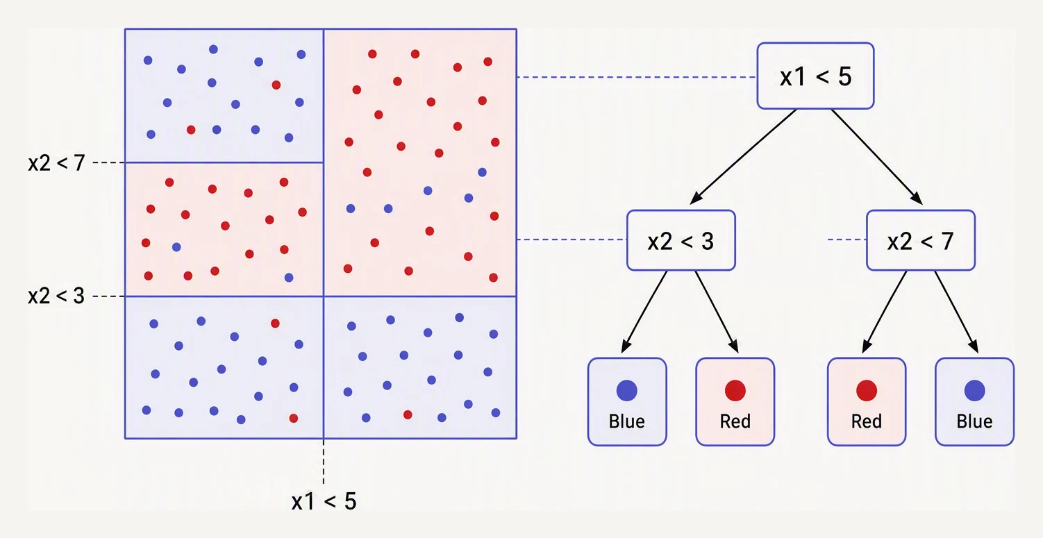
Every branch is one straight cut, always parallel to an axis.
At every node, the tree considers every feature and every possible split point, and picks the one that maximally separates the classes in the two resulting children. Impurity is how mixed a node’s class labels are — a perfectly pure node has only one class; a maximally impure node splits 50/50. The “how separated” is measured with one of:
- Gini impurity — the probability of misclassifying a random sample drawn from this node. Lower = purer.
- Entropy — the information content of the class distribution at this node. Lower = purer.
In practice they give nearly identical trees. Gini is the sklearn default because it’s slightly faster to compute. The greedy split-search keeps going recursively on each child until a stopping rule fires.
A split is chosen by how much it drops impurity. Trace one. Start with a node of 10
samples, 5 of each class — maximally impure. Split on feature ≤ t, sending 4 samples
(all class 0) left and 6 (1 class-0, 5 class-1) right:
| node | samples | class split | Gini |
|---|---|---|---|
| parent | 10 | 5 / 5 | 1 − (0.5² + 0.5²) = 0.500 |
| left child | 4 | 4 / 0 | 1 − (1² + 0²) = 0.000 |
| right child | 6 | 1 / 5 | 1 − ((1/6)² + (5/6)²) = 0.278 |
Weighted child impurity = (4/10)·0 + (6/10)·0.278 = 0.167, so this split drops
impurity by 0.500 − 0.167 = 0.333. The tree greedily tries every feature and every
threshold, and keeps whichever split drops impurity the most — then recurses on each
child. (Entropy gives nearly the same trees; Gini is just faster to compute.)
Fit a small tree on churn data
import numpy as np
import pandas as pd

from sklearn.tree import DecisionTreeClassifier, export_text
from sklearn.model_selection import train_test_split

rng = np.random.default_rng(0)
n = 300
df = pd.DataFrame({
    "logins_per_week":      rng.integers(0, 30, n),
    "support_tickets":      rng.integers(0, 8, n),
    "monthly_spend":        rng.gamma(2, 50, n).round(2),
    "days_since_last_login":rng.integers(0, 60, n),
})
df["churned"] = ((df["logins_per_week"] < 5) & (df["support_tickets"] >= 3)).astype(int)

X, y = df.drop(columns=["churned"]), df["churned"]
X_train, X_test, y_train, y_test = train_test_split(X, y, test_size=0.25, stratify=y, random_state=0)

tree = DecisionTreeClassifier(max_depth=3, random_state=0).fit(X_train, y_train)

print("test accuracy:", round(tree.score(X_test, y_test), 3))
print("\ntree structure:")
print(export_text(tree, feature_names=list(X.columns)))
Read the tree top-to-bottom. Each line is a question; each indent level is a step deeper. You can hand that printout to your product manager and they’ll understand it. No other model in ML offers this level of interpretability.
The hyperparameters that matter
A decision tree with no limits will grow until every training row sits in its own leaf — 100% training accuracy, terrible test accuracy. That’s the classic decision-tree failure mode. Three hyperparameters tame it:
| Parameter | What it does | Typical values |
|---|---|---|
max_depth | Hard cap on tree depth | 3 to 10 |
min_samples_split | Minimum rows in a node before it can be split | 10 to 50 |
min_samples_leaf | Minimum rows in a leaf | 5 to 20 |
These all do the same thing — stop the tree from growing too greedy.
max_depth is the lever you should reach for first.
import numpy as np

from sklearn.tree import DecisionTreeClassifier
from sklearn.model_selection import train_test_split

rng = np.random.default_rng(0)
X = rng.normal(size=(300, 5))
y = (X[:, 0] - X[:, 1] + 0.4 * rng.normal(size=300) > 0).astype(int)
X_tr, X_te, y_tr, y_te = train_test_split(X, y, test_size=0.3, stratify=y, random_state=0)

print(f"{'depth':>6}  {'train':>7}  {'test':>7}")
for d in [None, 1, 3, 5, 10, 20]:
    tr = DecisionTreeClassifier(max_depth=d, random_state=0).fit(X_tr, y_tr)
    print(f"{str(d):>6}  {tr.score(X_tr, y_tr):>7.3f}  {tr.score(X_te, y_te):>7.3f}")
You’ll see the classic pattern: shallow trees underfit (low train AND test), unconstrained trees overfit (perfect train, mediocre test), and somewhere in the middle is the sweet spot. Find it with cross-validation.
What trees are good at — and bad at
Good at:
- Interpretability. A 3-deep tree is a flowchart your colleagues can understand without statistics training.
- No feature scaling required. Splits are based on thresholds within each feature; the units don’t matter.
- Mixed feature types. Numeric and ordinal-encoded categorical features sit side by side without any extra effort.
- Non-linear relationships. Capture interactions naturally
(
if A > 5 and B < 2 then ...). - Robust to outliers. A few extreme values don’t shift a threshold much.
Bad at:
- High variance. Change a few training rows and the tree restructures entirely. This is the single biggest weakness.
- Smooth functions. Trees produce step-function predictions. If the
true relationship is
y = x², a tree approximates it with a staircase. - Extrapolation. Trees can only predict within the range of values they’ve seen.
That high-variance problem is what ensembles solve. A random forest averages many noisy trees to cancel out the noise. Gradient boosting fits a sequence of trees where each corrects its predecessor’s mistakes. Both routinely top tabular ML leaderboards.
Feature importance — but with a caveat
Every fitted tree exposes .feature_importances_, ranking features by
how much they reduce impurity across all splits. It’s a useful first
pass, but for serious analysis prefer permutation importance (shuffle
each feature on held-out data and measure the drop in score). Built-in
impurity-based importances are biased toward high-cardinality features.
from sklearn.inspection import permutation_importance
result = permutation_importance(tree, X_test, y_test, n_repeats=10, random_state=0)
In one breath
- A decision tree is a flowchart of if/else questions; at each node it greedily picks the feature + threshold that drops impurity (Gini or entropy) the most, then recurses.
- It’s the most interpretable model, needs no scaling, handles mixed types and non-linear interactions, and is robust to outliers.
- Its big weakness is high variance — a few changed rows restructure it; it also makes step-function predictions and can’t extrapolate.
- Tame overfitting with
max_depth(reach for first),min_samples_split,min_samples_leaf— an unbounded tree memorizes (100% train, poor test). .feature_importances_is a quick rank but biased toward high-cardinality features — prefer permutation importance. A single tree is a great debugging tool; the deployed model is an ensemble (random forest / gradient boosting).
Quick check
Quick check
Practice this in an interview
All questionsPruning regularizes a decision tree by preventing or removing branches that fit noise rather than a repeatable pattern. Pre-pruning stops growth with constraints such as maximum depth or minimum samples per leaf; post-pruning grows a larger tree and selects a smaller subtree, often with cross-validated cost-complexity penalty.
At each node, a decision tree evaluates eligible feature and threshold pairs, measures the weighted impurity left after the split, and chooses the pair with the largest impurity reduction. It repeats this greedy process on each child until a stopping rule or lack of useful split ends the branch.
Gini impurity uses squared class probabilities, while entropy uses logarithms to measure uncertainty. Both score weighted child purity and usually select similar splits; Gini is a little cheaper, but the data, class imbalance, and tree regularization matter more than the choice.
sklearn trees require numeric input and treat label-encoded integers as ordinal, which imposes a false ordering. One-hot encoding is correct but expensive for high-cardinality features. XGBoost (v2+) and LightGBM support native categorical splits that find the optimal binary partition of categories without ordinal assumptions.
Information gain measures how much a split reduces uncertainty (entropy) in the target variable. It is the difference between the parent node's entropy and the weighted average entropy of the child nodes. The split that maximises information gain is selected at each node.