The scikit-learn API
The fit, transform, and predict contract makes scikit-learn models, preprocessing, validation, and deployment compose cleanly.
Written and reviewed by Shreyash Prashu Last reviewed
What you'll learn
- Read the fit, transform, predict, and predict_proba contract without guessing what an estimator does
- Separate learned state from configuration, and understand why fit must see training data only
- Build leakage-resistant Pipelines and tune their nested parameters
- Route mixed numeric and categorical data with ColumnTransformer
- Diagnose the train-serve and shape errors that appear first in real sklearn projects
Before you start
At 3 a.m., a fraud model pages you. The model was trained on two numeric columns and worked beautifully in the notebook. The serving request still contains the merchant name, the production encoder was fitted on a different set of categories, and somebody scaled the test data before reporting accuracy.
Nothing is wrong with logistic regression. The surrounding code has quietly become three different programs.
Scikit-learn’s answer is a deliberately boring interface. A model, a scaler, an encoder, and a dimensionality reducer fit into the same workflow. Once you understand what each verb means, the library stops looking like a catalogue of unrelated classes and starts looking like Lego with strict instructions.
That shared design is the estimator pattern. An estimator is any scikit-learn object that learns something from data. A classifier is an estimator. So are StandardScaler, OneHotEncoder, PCA, and KMeans.
The mental model: configuration first, learning second
Suppose you create a scaler:
scaler = StandardScaler()It now has configuration—the default choice of centering and scaling—but has not seen your data. It does not know the average transaction amount.
Calling:
scaler.fit(X_train)makes it inspect the training data and store learned state. For a standard scaler, that includes one mean and one scale per feature. Calling:
X_train_scaled = scaler.transform(X_train)uses that state to convert values. It does not learn again.
This distinction is the API’s load-bearing wall:
- Configuration is chosen before fitting: a logistic regression’s
C, a tree’smax_depth, or an encoder’s unknown-category policy. - Learned state is calculated from data during
fit: coefficients, scaler means, or discovered categories. - Inference uses learned state on new data:
predict,predict_proba, andtransform.
Scikit-learn commonly marks learned attributes with a trailing underscore: scaler.mean_, model.coef_, or encoder.categories_. These values do not exist until fitting succeeds.
X conventionally means the feature matrix, with rows as examples and columns as variables. y means the target. If there are 10,000 transactions and 12 features, X.shape is (10000, 12) and a binary target usually has shape (10000,).
| Method | Meaning | Typical owners |
|---|---|---|
fit(X, y) | Learn from examples and targets | Supervised models |
fit(X) | Learn without targets | Scalers, clusterers, reducers |
transform(X) | Apply a learned feature conversion | Scalers, encoders, reducers |
predict(X) | Produce predictions | Regressors and classifiers |
predict_proba(X) | Produce class probabilities | Some classifiers |
fit_transform(X) | Fit, then transform the same data | Transformers |
This is a pattern, not a promise that every object has every method. A classifier normally has fit and predict; a scaler has fit and transform; KMeans has fit and predict, and can also provide labels through fit_predict.
fit_transform(X) means “learn from this data, then convert it.” It is not a leakage shield. Calling it on the full dataset before splitting still lets test examples influence preprocessing.
A small run, with the arithmetic exposed
Consider six card transactions. The model sees amount and age in hours. The target says whether the transaction was risky.
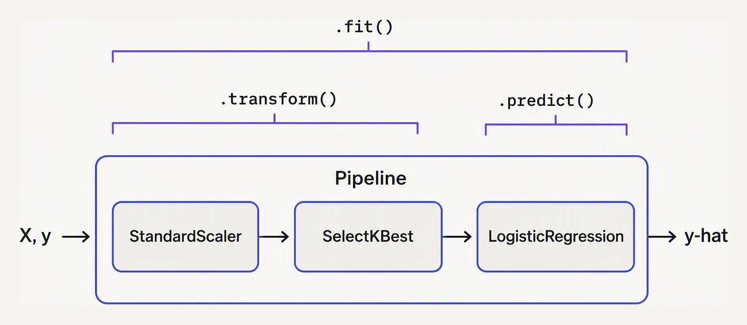
Learn the three verbs once and every estimator behaves the same.
import pandas as pd

from sklearn.model_selection import train_test_split
from sklearn.linear_model import LogisticRegression
from sklearn.preprocessing import StandardScaler

# Toy dataset: 6 transactions, 2 numeric features, binary label
df = pd.DataFrame({
    "amount":     [12.50, 850.00, 45.00, 2100.00, 9.99, 320.00],
    "hours_old":  [0.1,    23.0,   3.5,   71.0,   0.2,  12.0],
    "is_risky":   [0,      1,      0,     1,      0,    0],
})
X = df[["amount", "hours_old"]]
y = df["is_risky"]

X_train, X_test, y_train, y_test = train_test_split(
    X, y, test_size=0.33, random_state=0
)

scaler = StandardScaler().fit(X_train)
X_train_s = scaler.transform(X_train)
X_test_s = scaler.transform(X_test)

model = LogisticRegression().fit(X_train_s, y_train)

print("scaler.mean_ (learned on train):", scaler.mean_.round(2).tolist())
print("test predictions:", model.predict(X_test_s).tolist())
scaler.mean_ (learned on train): [743.12, 23.58]
test predictions: [0, 0]Why is the learned amount mean 743.12, rather than the mean of all six amounts? The random split puts four rows in training: amounts 850, 2100, 12.50, and 9.99. Their average is:
(850 + 2100 + 12.50 + 9.99) / 4 = 743.1225
The test rows remain unseen while the scaler learns. They are converted later using the training mean and training scale. The model receives transformed numbers, but the transformation has not peeked at the answers.
The model’s fit learns coefficients connecting scaled features to the risk label. At prediction time, model.predict applies those coefficients and returns class labels. Each object has one job, and manual code must remember the order.
Pipeline: make the whole recipe one estimator
A Pipeline is an ordered chain in which intermediate steps transform features and the final step makes predictions. It exposes its own .fit, .predict, and, when appropriate, .transform.
from sklearn.pipeline import Pipeline

pipe = Pipeline([
    ("scale", StandardScaler()),
    ("clf", LogisticRegression()),
])

pipe.fit(X_train, y_train)
predictions = pipe.predict(X_test)
pipe.fit does the following:
- Fits
scaleonX_train. - Transforms
X_trainwith that scaler. - Fits
clfon the transformed features.
Later, pipe.predict(X_test) transforms the test rows with the already-fitted scaler, passes them to the classifier, and returns predictions. It does not refit anything.
This matters during cross-validation. In five-fold validation, a correct workflow fits a fresh scaler on each fold’s training rows, then transforms that fold’s held-out rows. Manually scaling the whole matrix first allows held-out rows to influence the training calculation. The labels need not be exposed for evaluation to become contaminated. See train, test, and cross-validation and data leakage.
A pipeline also gives hyperparameter search one object to operate on. Nested parameter names use the step name, two underscores, and the parameter:
pipe.set_params(clf__C=0.1)A search can compare clf__C or replace the final estimator. Each candidate is refit inside each training fold instead of reusing preprocessing learned outside the fold.
Intermediate steps must provide fit and transform; the final step must provide fit and commonly predict. A classifier cannot normally sit in the middle because it predicts rather than transforming features for the next step.
A pipeline prevents leakage from its internal steps, but it cannot detect every leaky feature. If you create chargeback_resolved using information recorded after a transaction, placing that column in a perfect pipeline does not make it valid. The API can enforce a preprocessing boundary; it cannot know the future.
Mixed columns: ColumnTransformer
Fraud data usually mixes numeric fields such as amount and hours_old with categories such as merchant. A numeric scaler should not receive the word food, and a one-hot encoder should not treat 850.00 as a category.
ColumnTransformer applies different transformers to named subsets of columns, then concatenates the resulting blocks. Put it inside a pipeline so each branch is fitted only on training data.
import pandas as pd

from sklearn.compose import ColumnTransformer
from sklearn.pipeline import Pipeline
from sklearn.preprocessing import StandardScaler, OneHotEncoder
from sklearn.linear_model import LogisticRegression

df = pd.DataFrame({
    "amount":      [12.5, 850, 45, 2100, 9.99, 320, 75, 1500],
    "hours_old":   [0.1, 23, 3.5, 71, 0.2, 12, 1, 48],
    "merchant":    ["food", "elec", "food", "elec", "food", "ride", "food", "elec"],
    "is_risky":    [0, 1, 0, 1, 0, 0, 0, 1],
})
X = df.drop(columns=["is_risky"])
y = df["is_risky"]

pre = ColumnTransformer([
    ("num", StandardScaler(), ["amount", "hours_old"]),
    ("cat", OneHotEncoder(handle_unknown="ignore"), ["merchant"]),
])

pipe = Pipeline([
    ("pre", pre),
    ("clf", LogisticRegression()),
])

pipe.fit(X, y)
print(pipe.predict(pd.DataFrame([{
    "amount": 9.0,
    "hours_old": 0.5,
    "merchant": "food",
}])).tolist())
The numeric branch produces two scaled columns. The categorical branch discovers three merchant categories and creates indicator columns such as merchant_food, merchant_elec, and merchant_ride. The branches are joined into one matrix for logistic regression.
handle_unknown="ignore" prevents a new category such as "books" from raising an error at prediction time. The encoder emits zeros for the known merchant indicators. That keeps inference running, but does not mean the model understands books; decide whether this treatment is acceptable.
Columns not listed are dropped by default. remainder="passthrough" can carry them through unchanged, but use it deliberately. A raw string or ID column may cause an error or let the model memorize users and transactions.
One-hot encoding can produce a sparse matrix with many mostly-zero columns. That is often efficient, but some estimators require dense arrays. Check the estimator’s input support and category cardinality before converting to dense.
For feature inspection:
feature_names = pipe.named_steps["pre"].get_feature_names_out()These names reveal which transformed column reached the model.
The surrounding API: swapping, inspecting, and scoring
The shared interface makes experiments cheap. Replacing the final estimator can leave preparation unchanged:
from sklearn.ensemble import RandomForestClassifier

pipe.set_params(clf=RandomForestClassifier(random_state=0))
The interface is compatible, but preprocessing choices are not universal. Logistic regression benefits from scaling; a random forest usually does not need it because it splits on thresholds.
pipe.named_steps["clf"] retrieves a fitted step, while get_params() exposes configuration and nested parameters for tools such as GridSearchCV.
Be careful with .score(). For a classifier it is commonly accuracy; for a regressor it is commonly R². Neither is automatically the metric your product needs. A fraud model can achieve high accuracy by predicting “safe” whenever fraud is rare. Choose an explicit metric such as average precision, recall at a review budget, or expected cost. See the metrics lesson.
At the model boundary, save one fitted pipeline rather than separate scaler, encoder, feature-list, and model files. This reduces train-serve ordering mistakes. Serialization still has costs: pickle-based formats can execute code when loaded, and Python, scikit-learn, NumPy, and dependency versions should be controlled.
What fails first
| First symptom | Likely cause | Fix |
|---|---|---|
NotFittedError or missing mean_ | transform or predict ran before successful fit | Fit the estimator or load a fitted pipeline |
could not convert string to float | A categorical column reached a numeric estimator | Encode, drop, or use a suitable representation |
Found unknown categories ... | A new category met the encoder’s default error policy | Choose handle_unknown="ignore" or an unknown bucket |
| Validation looks brilliant, production collapses | Leakage or train-serve preprocessing mismatch | Fit learned preprocessing inside the pipeline and validate the serving schema |
X has 7 features ... expecting 8 | Training and inference produced different columns | Persist the fitted encoder and pass the same raw schema |
| Memory use explodes after adding a category | One-hot encoding created a huge matrix or was densified | Inspect cardinality and sparsity; reduce or choose a compatible estimator |
Which tool should hold the logic?
| Situation | Use | Reason |
|---|---|---|
| Transformations happen one after another | Pipeline | One ordered fit boundary |
| Different columns need different preparation | ColumnTransformer inside Pipeline | Parallel branches are combined safely |
| You want a simple chain without naming steps | make_pipeline | It creates automatic names |
| You need to search preprocessing and model choices | Pipeline plus a search tool | Names such as clf__C refit the whole recipe |
If a transformation is fixed arithmetic that uses no data, it may not need an estimator. If the data is already clean and the model needs no preprocessing, a bare estimator is reasonable.
The trade-off is abstraction: a pipeline can hide intermediate arrays while debugging. Inspect named_steps, transform a small sample, and check shapes and feature names. More structure reduces accidental inconsistencies, but you must learn where to look.
In one breath
- An estimator stores configuration in its constructor and creates learned state during
fit. transformapplies learned preparation;predictproduces outputs;predict_probaproduces supported class probabilities.- Fit every data-dependent step on training data only.
- A Pipeline chains preparation and prediction behind one interface and refits each learned step inside each cross-validation fold.
- A ColumnTransformer routes named column groups through different branches.
handle_unknown="ignore"keeps unseen categories from crashing inference, but does not teach the model their meaning..score()is a convenience, not necessarily the right business metric.- Pipelines reduce leakage and train-serve skew, but cannot rescue a feature defined with future information.
Quick check
Quick check
X_train only, not on X_train + X_test?pipe.fit(X_train, y_train). What does pipe.predict(X) do?OneHotEncoder(handle_unknown="ignore") inside a ColumnTransformer. What should happen?Practice this in an interview
All questionsK-means partitions n points into k clusters by alternating between two steps: assigning each point to its nearest centroid, then recomputing each centroid as the mean of its assigned points. It repeats until assignments stop changing, which guarantees convergence but not a globally optimal solution.
Standardization rescales features to zero mean and unit variance; normalization squashes values into a fixed range, usually [0, 1]. Distance-based and gradient-based models are sensitive to scale and require one of these; tree-based models split on rank order and are scale-invariant.
ML CI/CD must validate not just code correctness but also model quality — automated retraining triggers, data validation, model evaluation gates, and canary deployment checks that standard software pipelines have no equivalent for. A regression in model AUC is as much a deployment failure as a 500 error.
A data contract is an explicit, enforced agreement between a data producer and consumers that specifies schema, types, semantics, and quality or freshness expectations, plus rules for how it can evolve. It prevents silent breakage by validating data at ingestion so violations are caught and quarantined or alerted instead of flowing into the model. Combined with a schema registry and backward-compatible evolution rules, it lets producers change data without unexpectedly corrupting downstream features and predictions.