PyTorch in 5 minutes
A practical PyTorch quickstart: tensors, autograd, devices, dtypes, and the training loop behind every neural network.
Written and reviewed by Shreyash Prashu Last reviewed
What you'll learn
- What a tensor is and how shape, dtype, and device determine what operations are possible
- How autograd builds a computation graph and computes gradients with the chain rule
- The five steps of a PyTorch training loop, including why gradients must be cleared
- How to move a model and its batches safely between CPU, CUDA, and Apple Silicon
- How to distinguish training mode, evaluation mode, and gradient-free inference
Before you start
Your first PyTorch bug usually arrives before the model has learned anything.
You create a tensor from a Python list. It turns out to be an integer tensor. Your model’s weights are floating-point tensors. A matrix multiplication fails with a message about Long and Float.
Or the model is on the GPU while one batch is still on the CPU. PyTorch refuses to guess whether you intended to copy 4 kilobytes or 4 gigabytes.
Or the loss gets larger every step because the gradients from yesterday’s batch are still sitting on the parameters.
PyTorch exists to make the useful part easy: describe a computation, ask for its gradients, and update the weights. It also makes the boundaries visible. Shape, dtype, and device determine whether the computation is meaningful and whether it can run at all.
Tensors are arrays with a backstory
A tensor is a multidimensional array that also carries a dtype, a device, and optional gradient-tracking information:
PyTorch is NumPy-shaped data plus automatic differentiation and hardware acceleration.
You will inspect these three attributes constantly:
- Shape says how many values exist along each axis.
- Dtype says how each value is represented, such as 32-bit floating point or 64-bit integer.
- Device says where the values live: usually
cpu,cuda, ormps.
import torch

x = torch.tensor([[1.0, 2.0], [3.0, 4.0]])
print(x.shape)        # torch.Size([2, 2])
print(x.dtype)        # torch.float32
print(x.device)       # cpu
This tensor has two rows and two columns, uses four bytes per value, and is stored in CPU memory. A CUDA tensor lives in GPU memory instead. Operations involving tensors on different devices would require a transfer, so PyTorch makes you request that transfer explicitly.
Shape errors are equally literal. A tensor with shape [64, 1] contains 64 examples with one feature each; [64, 10] contains 64 examples with ten features. They are not interchangeable just because both are batches.
PyTorch follows NumPy broadcasting rules for many elementwise operations. In x @ w + b, shapes [64, 1], [1, 1], and [1] produce [64, 1]; the one bias value is broadcast across all 64 rows.
Do not convert every tensor to floating point automatically. Classification targets are often integer class IDs, while regression targets for mean squared error are normally floating point. The correct dtype depends on the tensor’s role.
You can read more about the gradient engine in autograd. The key question is how PyTorch knows which direction to change a weight.
Autograd records the route to the loss
Suppose a model predicts a house price:
prediction = x * w + bFor x = 3, w = 2, and b = 1, the prediction is 7. If the correct scaled price is 8, a loss function turns that error into a scalar the optimizer can reduce.
The derivative with respect to w answers this question:
If
wincreases slightly, how does the loss change?
For a two-parameter model, you could apply the chain rule by hand. For a model with millions of parameters, autograd handles the bookkeeping.
When a tensor has requires_grad=True, PyTorch records operations involving it while gradient tracking is enabled. Each operation contributes a node to a computation graph, which stores enough intermediate values to apply the chain rule later:
w, x ── multiply ── prediction ── loss
b ───────── add ────┘
Calling loss.backward() walks the graph backward. It computes derivatives for tracked parameters and stores them in each parameter’s .grad attribute. A gradient has the same shape as its parameter.
The optimizer is separate: it reads those stored gradients and changes the parameters. For stochastic gradient descent:
new weight = old weight - learning rate × gradientA positive gradient generally means decreasing the weight will reduce the loss; a negative gradient means increasing it may help. The learning rate controls the step size.
Autograd tracks numerical operations, not meaning. It does not know whether a tensor represents an image, sentence, or price. A mathematically valid gradient can still be useless if the data or loss is wrong.
The graph is normally rebuilt for each training step and released after backward. PyTorch retains intermediate activations during the current forward pass because backward needs them, which is why large models can run out of GPU memory even when their parameters fit.
The training loop, in five steps
Here is the basic heartbeat:
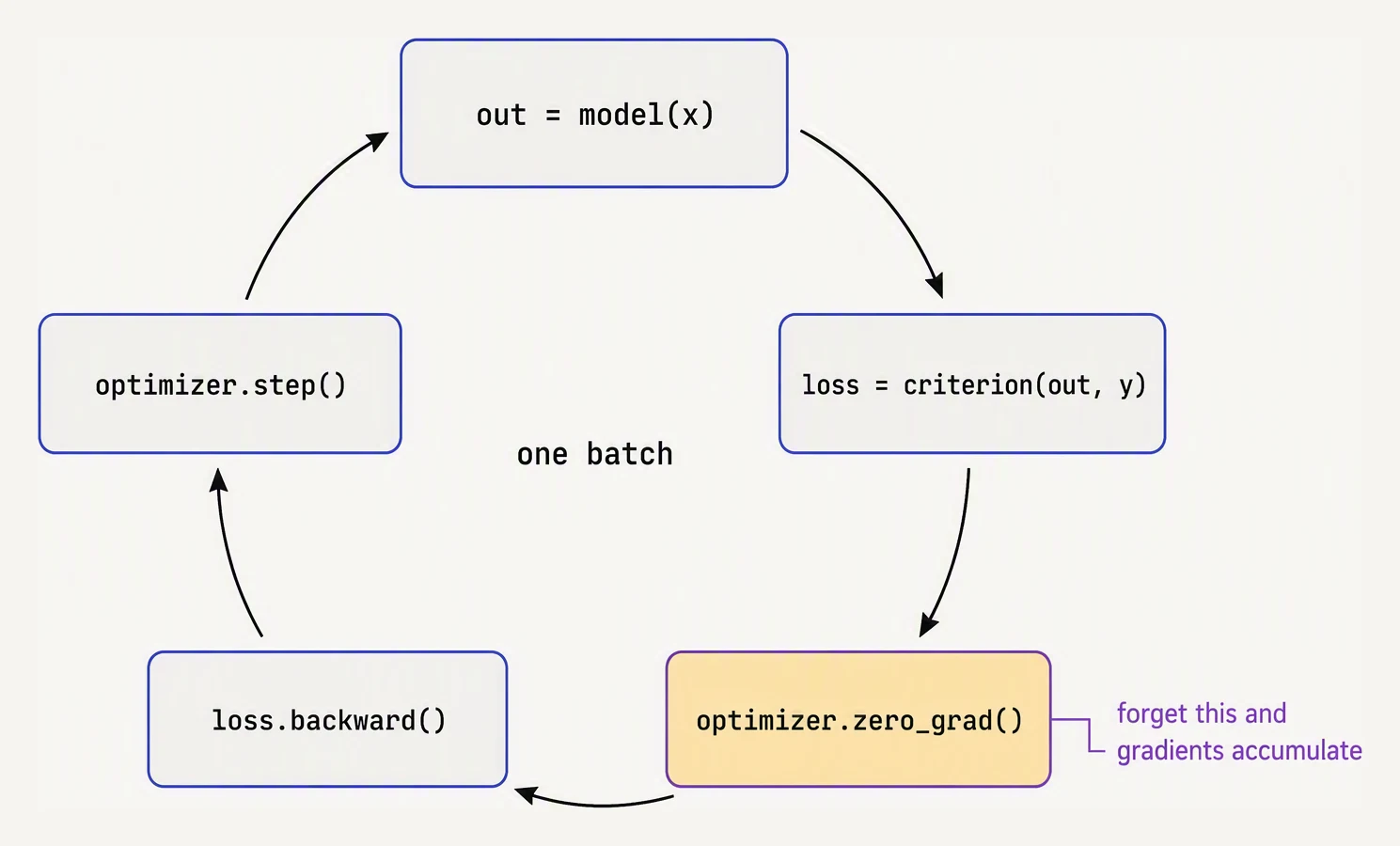
Every PyTorch script you will ever read is this loop with more decoration.
pred = model(x)              # 1. forward pass
loss = loss_fn(pred, y)      # 2. measure the error
optimizer.zero_grad()        # 3. clear previous gradients
loss.backward()              # 4. compute new gradients
optimizer.step()             # 5. update parameters
Clearing gradients before the forward pass is easy to read, but this is also valid:
loss.backward()
optimizer.step()
optimizer.zero_grad()
The rule is to clear gradients before accumulating the next update. .backward() adds to existing .grad values; it does not replace them. If batch one produces a gradient of 2 and batch two produces 3, forgetting to clear the first makes the second update use 5.
That accumulation is useful when deliberately combining several small batches into one update. Delay optimizer.step() and zero_grad() for the accumulation cycle, and scale each loss if you want to preserve the mean-loss gradient. Ordinary one-update-per-batch training clears gradients every iteration.
This is a complete model:
import torch
import torch.nn as nn

# 64 examples, one feature each.
x = torch.randn(64, 1)
y = 2.0 * x + 1.0 + 0.1 * torch.randn(64, 1)

model = nn.Linear(1, 1)
loss_fn = nn.MSELoss()
optimizer = torch.optim.SGD(model.parameters(), lr=0.1)

model.train()

for step in range(200):
    optimizer.zero_grad()

    pred = model(x)
    loss = loss_fn(pred, y)

    loss.backward()
    optimizer.step()

print(model.weight.item(), model.bias.item())
nn.Linear(1, 1) contains one weight and one bias. model.parameters() returns those trainable tensors. MSELoss squares prediction errors and averages them.
Because the generated data follows y = 2x + 1 with small noise, the learned weight should approach 2 and the bias should approach 1. It will not be exact: the data is noisy, initialization is random, and 200 steps is a small experiment.
The optimizer receives parameter references, not the model architecture. That separation lets you swap SGD for AdamW without changing the model’s forward pass. See optimizers.
Real training uses batches
The previous example uses all 64 examples for every update. That is full-batch training. Neural networks usually use mini-batches, such as 32 or 256 examples.
Mini-batches make updates cheaper and add noise to the gradient. That noise can help optimization, but each update is less exact. Batch size and learning rate interact, so changing one may require reconsidering the other.
for xb, yb in train_loader:
    xb = xb.to(device)
    yb = yb.to(device)

    optimizer.zero_grad()
    pred = model(xb)
    loss = loss_fn(pred, yb)
    loss.backward()
    optimizer.step()
If xb has shape [32, 10], it contains 32 examples with 10 features each. The data loader supplies tensors; the model and loss create the computation graph.
Device: move the computation, not just the model
The model and every tensor used with it must be on compatible devices.
device = torch.device("cpu")

if torch.cuda.is_available():
    device = torch.device("cuda")
elif torch.backends.mps.is_available():
    device = torch.device("mps")

model = nn.Linear(1, 1).to(device)
x = x.to(device)
y = y.to(device)
Move the model once before training and move each batch as it arrives. Moving a tiny regression to a GPU may be slower than using a CPU because transfer and kernel-launch overhead outweigh the small computation.
When debugging, inspect one representative object before reading a long stack trace:
print(next(model.parameters()).device)
print(x.device)
print(x.dtype, x.shape)
Training mode is not inference mode
Some layers behave differently during training and evaluation. Dropout removes random activations during training, while batch normalization uses batch statistics during training and stored statistics during evaluation.
Call model.train() before training and model.eval() before validation or prediction:
model.eval()

with torch.no_grad():
    predictions = model(x)
model.eval() changes layer behavior; it does not disable autograd. torch.no_grad() prevents graph construction and reduces memory use when gradients are unnecessary.
A validation pass therefore looks like this:
model.eval()

with torch.no_grad():
    validation_pred = model(validation_x)
    validation_loss = loss_fn(validation_pred, validation_y)

model.train()
Forgetting eval() can make validation metrics fluctuate because dropout remains active. Forgetting no_grad() usually produces correct predictions but wastes memory and computation.
When the loop goes sideways
Size or shape errors. Print x.shape, pred.shape, and y.shape. In regression, predictions and targets should normally match. A prediction shaped [32, 1] and a target shaped [32] may broadcast into a loss while comparing the wrong pairs.
Long and Float errors. Inspect .dtype. Convert features to float32, but keep class-index targets in the dtype required by the chosen classification loss.
nan loss. Check inputs for nan or infinity, reduce an excessive learning rate, and inspect for exploding activations or unstable operations.
Zero gradients or a loss that does not improve. Training may be inside no_grad(), the prediction may have been detached, or the learning rate may be unsuitable. After backward, inspect:
loss.backward()
print(model.weight.grad)
A None gradient means no gradient reached that parameter. A tensor of zeros means the graph exists but produced no useful local signal.
A growing loss. The learning rate may be too large, or gradients may be accumulating because zero_grad() is missing. Learning rates are not universal: parameter scales, input scales, and loss curvature matter.
The honest boundary
PyTorch removes derivative bookkeeping, not the need to choose suitable data, objectives, architectures, dtypes, devices, learning rates, and evaluation procedures.
It also has costs. Autograd stores intermediate values, Python-level model code can add overhead, and CPU–GPU transfers are not free. For a small fixed numerical program, NumPy may be simpler. At larger scales, memory strategy, precision, batching, and distributed execution become important engineering decisions.
The basic model remains stable:
- Tensors hold values with shape, dtype, and device.
- The forward pass builds a computation.
- The loss measures wrongness.
- Autograd applies the chain rule backward.
- The optimizer changes parameters.
- The next batch starts with fresh gradients.
In one breath
- A tensor is an array plus metadata and optional gradient tracking.
- Shape determines how operations line up; dtype determines representation; device determines where they run.
- Autograd records operations involving trainable tensors and applies the chain rule when
loss.backward()runs. - An optimizer reads
.gradand updates parameters. - The standard loop is forward, loss, zero gradients, backward, and optimizer step.
- Gradients accumulate by default, so ordinary training must clear them.
- Put the model, inputs, targets, and masks on compatible devices.
- Use
model.train()for training,model.eval()for evaluation, andtorch.no_grad()when gradients are unnecessary.
Quick check
Quick check
optimizer.zero_grad() every training step?model(x)?[32, 10], but your target tensor has shape [32] and dtype float32. What should you inspect first?Practice this in an interview
All questionsThe forward pass transforms an input through each layer’s learned parameters and activation functions into an output, then training compares that output with the label to compute a loss. The framework records the operations and needed intermediate values so backpropagation can calculate gradients, while inference normally skips that graph.
Neural network training is dominated by large matrix multiplications that are embarrassingly parallel. GPUs have thousands of small cores optimised for this exact operation, whereas CPUs have tens of powerful cores optimised for low-latency sequential logic. The throughput difference is 10–100x for typical DL workloads.
A transformer encoder turns token embeddings into contextual representations by repeating self-attention, residual connections, layer normalisation, and a position-wise feed-forward network. The original block is post-normalised, while many deeper implementations use pre-normalisation, so the order is an important implementation detail.
Transformers usually outperform recurrent neural networks because they train all sequence positions in parallel, connect distant tokens through short attention paths, and scale effectively with modern accelerator hardware. Their quadratic attention and growing context memory still make RNNs attractive for streaming and highly resource-constrained workloads.